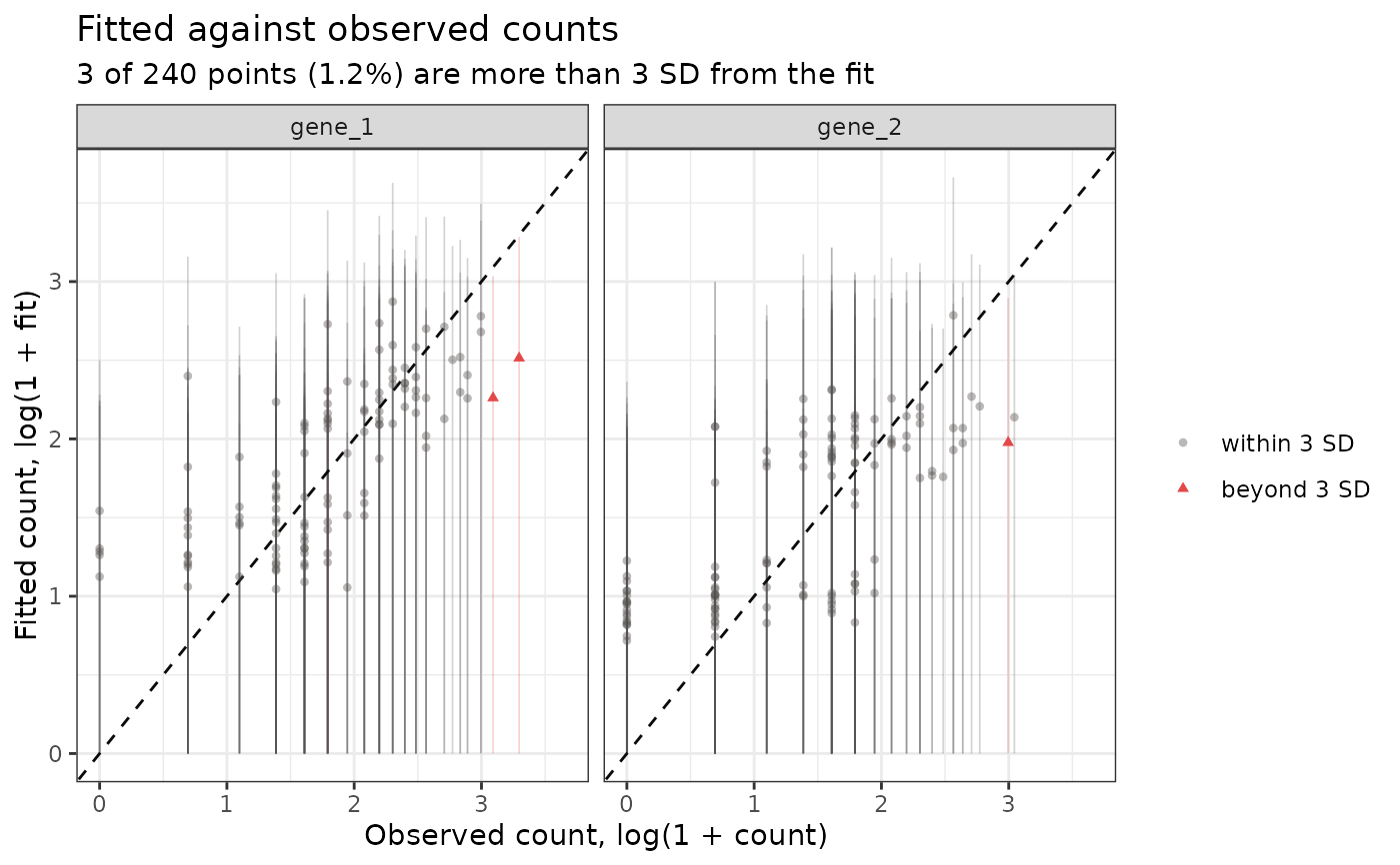
Plot the fitted count against the observed count — plot_fitted_vs

A diagnostic of whether the over-dispersion accounts for how far the counts lie from the fit. Each point is one cell and one gene. The x-axis is the observed count $A_{ji}$ and the y-axis the fitted count $m_{ji} = \ell_{ji}\mu_{ji}$, both drawn as $\log(1 + \cdot)$, so a count that equals its fit is on the line $y = x$. Under the model $A_{ji}$ is negative binomial with mean $m_{ji}$ and variance $m_{ji}(1 + \ell_{ji}/\beta_j)$, and a point is drawn in red when its count is more than num_sd standard deviations from its fit.

Usage

plot_fitted_vs_observed(
  input_obj,
  bool_draw_bars = FALSE,
  genes = NULL,
  max_points = 50000,
  num_sd = 3,
  seurat_obj = NULL,
  seed_number = 10
)

Arguments

input_obj: eSVD object after estimate_nuisance.
bool_draw_bars: If TRUE, draw each point's bar. Default FALSE.
genes: NULL, for all the genes, or a character vector of genes, each drawn in its own panel with all of its cells.
max_points: When genes is NULL, the largest number of points to draw. If there are more pairs of a cell and a gene than this, that many are sampled; the fitted count is computed for the sampled pairs only, so no cell-by-gene matrix is allocated.
num_sd: One positive number, the number of standard deviations beyond which a point is red.
seurat_obj: NULL, or the Seurat object the analysis was run on. Required when input_obj has no counts (it was built with bool_diet = TRUE); see recompute_pvalue.
seed_number: Seed for the sample of pairs; NULL leaves the random number stream alone.

Value

A ggplot object. Its data has one row per point and columns cell, gene, observed, fitted, sd, bool_outside (is the point red?), status (the same, as the factor the legend is drawn from), and the coordinates drawn: log_observed, log_fitted, log_lower and log_upper (the ends of the bar). The share of red points is mean(plot$data$bool_outside).

Details

With bool_draw_bars = TRUE each point carries a vertical bar, the interval $m_{ji} \pm$ num_sd standard deviations (truncated at zero), drawn along the y-axis at the observed count. A point is red exactly when its bar does not reach the line $y = x$.

What to look for. The points should follow the line, and only a small share should be red. With num_sd = 3, counts simulated from the model and drawn with their true rates gave a share of 1 to 2 percent, more than the 0.3 percent of a Gaussian because a count is skewed to the right. A rate ten times too large gave about 5 percent, and a rate ten times too small under 0.1 percent. So a larger share, or bars that are systematically too short to reach the line, means the over-dispersion is underestimated (the rate is too large), and bars that reach far past the line with almost no red point mean it is overestimated. Points that leave the line together, on one side, are a problem of the fit and not of the over-dispersion.

The rate is nuisance_vec, the rate after the cap and before the adjustments compute_posterior makes to it, and the library size is the one estimate_nuisance used.

Examples

set.seed(10)
sim <- generate_null(cell_per_person = 15, num_genes = 40,
                     num_individuals = 8)
esvd_obj <- initialize_esvd(dat = sim$obs_mat,
                            covariates = sim$covariates,
                            metadata_individual = sim$metadata_individual,
                            case_control_variable = "CC",
                            bool_intercept = TRUE,
                            k = 2,
                            lambda = 0.1)
esvd_obj <- reparameterization_esvd_covariates(input_obj = esvd_obj,
                                               fit_name = "fit_Init",
                                               omitted_variables = "Log_UMI")
esvd_obj <- opt_esvd(input_obj = esvd_obj,
                     max_iter = 5,
                     offset_variables = setdiff(colnames(esvd_obj$covariates), "CC"),
                     fit_name = "fit_First",
                     fit_previous = "fit_Init")
esvd_obj <- reparameterization_esvd_covariates(input_obj = esvd_obj,
                                               fit_name = "fit_First",
                                               omitted_variables = "Log_UMI")
esvd_obj <- estimate_nuisance(input_obj = esvd_obj)
if(requireNamespace("ggplot2", quietly = TRUE)){
  plot1 <- plot_fitted_vs_observed(input_obj = esvd_obj,
                                   genes = colnames(sim$obs_mat)[1:2],
                                   bool_draw_bars = TRUE)
  plot(plot1)
  mean(plot1$data$bool_outside)
}

#> [1] 0.0125