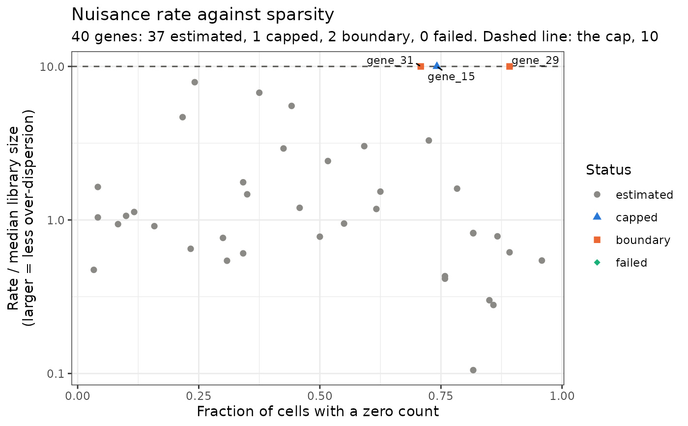
Plot each gene's nuisance rate against a summary of the gene

A diagnostic of the over-dispersion. Each point is a gene. The y-axis is the gene's unit-free rate, its Gamma rate divided by the median over cells of its library size, \(\hat\beta_j / \mathrm{median}_i\, \ell_{ji}\), on a \(\log_{10}\) scale. A larger value means less over-dispersion. The cap of estimate_nuisance is the same number for every gene on this scale, and is drawn as a dashed line at cap_multiplier; the genes it acted on sit on the line.

Usage

plot_nuisance(
  input_obj,
  x_axis,
  bool_uncapped = FALSE,
  genes = NULL,
  num_label = 10
)

Arguments

input_obj: eSVD object after estimate_nuisance (version 1.2.0 or later), and after the test when x_axis = "log10pvalue".
x_axis: One of "mean_expression" (the gene's mean count over cells, \(\log_{10}\) scale), "log10pvalue" (\(-\log_{10}\) of its p-value) or "sparsity" (the fraction of cells in which its count is zero).
bool_uncapped: If TRUE, draw the rate before the cap (nuisance_mle_vec). Default FALSE, the rate the analysis used.
genes: NULL, or a character vector of genes to label.
num_label: When genes is NULL, how many genes to label: the genes whose status is not estimated, in decreasing order of \(-\log_{10}\) p-value (or of the rate before the cap, if the object has not been tested). 0 labels none.

Value

A ggplot object. Its data has one row per analyzed gene, in the order of the fit, and columns gene, x_value, unit_free_rate, nuisance_status and bool_label.

Details

What to look for. Most genes should be estimated, below the line. A large share at the line means the cap, and not the data, is setting the over-dispersion. Against "mean_expression" and "sparsity", the genes at the line are expected among the lowly expressed and the sparse, whose counts carry little information about the rate. Against "log10pvalue", the genes with the smallest p-values should not be predominantly the ones at the line: a gene whose rate is very large has a posterior that follows the fit, and an inflated statistic. Drawing the plot with bool_uncapped = TRUE shows how far above the line the rates were.

The function needs neither the counts nor the covariates, so it works on an object built with bool_diet = TRUE. Genes that were not analyzed (the all-zero genes eSVD_helper reinserts) are not drawn.

Examples

set.seed(10)
sim <- generate_null(cell_per_person = 15, num_genes = 40,
                     num_individuals = 8)
esvd_obj <- initialize_esvd(dat = sim$obs_mat,
                            covariates = sim$covariates,
                            metadata_individual = sim$metadata_individual,
                            case_control_variable = "CC",
                            bool_intercept = TRUE,
                            k = 2,
                            lambda = 0.1)
esvd_obj <- reparameterization_esvd_covariates(input_obj = esvd_obj,
                                               fit_name = "fit_Init",
                                               omitted_variables = "Log_UMI")
esvd_obj <- opt_esvd(input_obj = esvd_obj,
                     max_iter = 5,
                     offset_variables = setdiff(colnames(esvd_obj$covariates), "CC"),
                     fit_name = "fit_First",
                     fit_previous = "fit_Init")
esvd_obj <- reparameterization_esvd_covariates(input_obj = esvd_obj,
                                               fit_name = "fit_First",
                                               omitted_variables = "Log_UMI")
esvd_obj <- estimate_nuisance(input_obj = esvd_obj)
if(requireNamespace("ggplot2", quietly = TRUE) &&
   requireNamespace("ggrepel", quietly = TRUE)){
  plot1 <- plot_nuisance(input_obj = esvd_obj, x_axis = "sparsity")
  plot(plot1)
}