Analysis of CITE-seq
bm.RmdWe go through how to analyze single-cell multiomic data in this
vignette (RNA and Protein, via surface antibody markers). We focus on
the CITE-seq data, which comes directly from the SeuratData
package. (In fact, this dataset is showcased in https://satijalab.org/seurat/articles/weighted_nearest_neighbor_analysis.)
Preliminary analysis
Installing and loading the data
To install the data, uncomment the
SeuratData::InstallData("bmcite") line.
# SeuratData::InstallData("bmcite")
bm <- SeuratData::LoadData(ds = "bmcite")
This load in a dataset which 30,672 cells. In the RNA modality, there are 17,009 genes. In the ADT modality, there are 25 surface antibody markers.
Basic preprocessing of the data
We first preprocess the RNA modality. This results in 2000 highly
variable genes, and the PCA of the RNA modality is stored in the
pca slot.
Seurat::DefaultAssay(bm) <- 'RNA'
bm <- Seurat::NormalizeData(bm)
bm <- Seurat::FindVariableFeatures(bm)
bm <- Seurat::ScaleData(bm)
bm <- Seurat::RunPCA(bm,
                     verbose = F)
Next, we preprocess the ADT modality. We treat all 25 surface
antibody markers as the highly variable genes, and the PCA of the RNA
modality is stored in the apca slot.
Seurat::DefaultAssay(bm) <- 'ADT'
Seurat::VariableFeatures(bm) <- rownames(bm[["ADT"]])
bm <- Seurat::NormalizeData(bm,
                            normalization.method = 'CLR',
                            margin = 2)
bm <- Seurat::ScaleData(bm)
bm <- Seurat::RunPCA(bm,
                     npcs = 18,
                     reduction.name = 'apca',
                     verbose = F)
Basic analysis of the data
To illustrate what WNN does (which illustrates the “union of information”), we can also run WNN on this dataset.
set.seed(10)
bm <- Seurat::FindMultiModalNeighbors(
  bm,
  reduction.list = list("pca", "apca"),
  dims.list = list(1:30, 1:18),
  modality.weight.name = "RNA.weight"
)
Now, we are ready to visualize the data. To do this, we run three
different UMAPS, one for RNA, one for ADT, and one for the WNN (which
combines both the RNA and ADT modality). These are stored as
rna.umap, adt.umap, and wnn.umap
respectively.
set.seed(10)
bm <- Seurat::RunUMAP(bm,
                      reduction = 'pca',
                      dims = 1:30, assay = 'RNA',
                      reduction.name = 'rna.umap',
                      reduction.key = 'rnaUMAP_')
set.seed(10)
bm <- Seurat::RunUMAP(bm,
                      reduction = 'apca',
                      dims = 1:18, assay = 'ADT',
                      reduction.name = 'adt.umap',
                      reduction.key = 'adtUMAP_')
set.seed(10)
bm <- Seurat::RunUMAP(bm,
                      nn.name = "weighted.nn",
                      reduction.name = "wnn.umap",
                      reduction.key = "wnnUMAP_")
We are now ready to plot the data. We first need to set up an appropriate color palette.
col_palette <- c(
  "CD14 Mono" = rgb(255, 108, 145, maxColorValue = 255),
  "CD16 Mono" = rgb(255, 104, 159, maxColorValue = 255),
  "CD4 Memory" = rgb(231, 134, 26, maxColorValue = 255),
  "CD4 Naive"= rgb(224, 139, 0, maxColorValue = 255),
  "CD56 bright NK" = rgb(0.7, 0.7, 0.7),
  "CD8 Effector_1" = rgb(2, 190, 108, maxColorValue = 255),
  "CD8 Effector_2" = rgb(0, 188, 89, maxColorValue = 255),
  "CD8 Memory_1" = rgb(57, 182, 0, maxColorValue = 255),
  "CD8 Memory_2" = rgb(0, 186, 66, maxColorValue = 255),
  "CD8 Naive" = rgb(1, 184, 31, maxColorValue = 255),
  "cDC2" = rgb(255, 98, 188, maxColorValue = 255),
  "gdT" = rgb(133, 173, 0, maxColorValue = 255),
  "GMP" = rgb(255, 97, 201, maxColorValue = 255),
  "HSC" = rgb(247, 99, 224, maxColorValue = 255),
  "LMPP" = rgb(240, 102, 234, maxColorValue = 255),
  "MAIT" = rgb(149, 169, 0, maxColorValue = 255),
  "Memory B" = rgb(0, 180, 239, maxColorValue = 255),
  "Naive B" = rgb(2, 165, 255, maxColorValue = 255),
  "NK" = rgb(0.6, 0.6, 0.6),
  "pDC" = rgb(255, 101, 174, maxColorValue = 255),
  "Plasmablast" = rgb(1, 191, 196, maxColorValue = 255),
  "Prog_B 1" = rgb(172, 136, 255, maxColorValue = 255),
  "Prog_B 2" = rgb(121, 151, 255, maxColorValue = 255),
  "Prog_DC" = rgb(252, 97, 213, maxColorValue = 255),
  "Prog_Mk" = rgb(231, 107, 243, maxColorValue = 255),
  "Prog_RBC" = rgb(220, 113, 250, maxColorValue = 255),
  "Treg" = rgb(243, 123, 89, maxColorValue = 255)
)

p1 <- Seurat::DimPlot(bm,
                      reduction = "rna.umap",
                      group.by = "celltype.l2",
                      cols = col_palette,
                      label = T, repel = T, label.size = 2.5)
p1 <- p1 + Seurat::NoLegend()
p1 <- p1 + ggplot2::ggtitle("RNA") + ggplot2::labs(x = "", y = "")
p1 <- p1 + ggplot2::theme(legend.text = ggplot2::element_text(size = 5))

p2 <- Seurat::DimPlot(bm,
                      reduction = "adt.umap",
                      group.by = "celltype.l2",
                      cols = col_palette,
                      label = T, repel = T, label.size = 2.5)
p2 <- p2 + Seurat::NoLegend()
p2 <- p2 + ggplot2::ggtitle("ADT") + ggplot2::labs(x = "", y = "")
p2 <- p2 + ggplot2::theme(legend.text = ggplot2::element_text(size = 5))

p3 <- Seurat::DimPlot(bm,
                      reduction = "wnn.umap",
                      group.by = "celltype.l2",
                      cols = col_palette,
                      label = T, repel = T, label.size = 2.5)
p3 <- p3 + Seurat::NoLegend()
p3 <- p3 + ggplot2::ggtitle("WNN") + ggplot2::labs(x = "", y = "")
p3 <- p3 + ggplot2::theme(legend.text = ggplot2::element_text(size = 5))

p_all <- cowplot::plot_grid(p1, p2, p3, ncol = 3)
p_all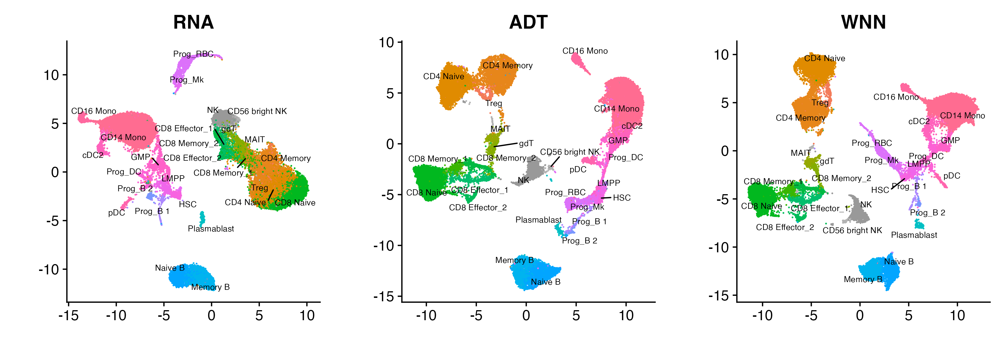
UMAPs of the RNA modality (left), ADT modality (middle), or WNN (right, which combines the information in the RNA and ADT)
Running Tilted-CCA
We are now ready to run Tilted-CCA.
Hard clustering the cells
Based on the visualizations, we assess that there is obvious clustering structure in the data (which we could’ve assessed if the data did not have cell type labels). Hence, we would like to pass “hard clusters” (one clustering for each modality) into Tilted-CCA to get more informative common and distinct embeddings. This results in 11 clusters for the RNA modality, and 14 communities for the ADT modality.
Seurat::DefaultAssay(bm) <- "RNA"
set.seed(10)
bm <- Seurat::FindNeighbors(bm, dims = 1:30)
bm <- Seurat::FindClusters(bm, resolution = 0.25)

Seurat::DefaultAssay(bm) <- "ADT"
set.seed(10)
bm <- Seurat::FindNeighbors(bm, dims = 1:18, reduction = "apca")
bm <- Seurat::FindClusters(bm, resolution = 0.25)
We can plot the clusters. This is a way to assess if the clustering from each modality is appropriate prior to using Tilted-CCA.
p1 <- Seurat::DimPlot(bm,
                      reduction = "rna.umap",
                      group.by = "RNA_snn_res.0.25",
                      label = TRUE, label.size = 2.5)
p1 <- p1 + Seurat::NoLegend() + ggplot2::labs(x = "", y = "")
p1 <- p1 + ggplot2::ggtitle("RNA clustering")
p1 <- p1 + ggplot2::theme(legend.text = ggplot2::element_text(size = 5))

p2 <- Seurat::DimPlot(bm,
                      reduction = "adt.umap",
                      group.by = "ADT_snn_res.0.25",
                      label = TRUE, label.size = 2.5)
p2 <- p2 + Seurat::NoLegend() + ggplot2::labs(x = "", y = "")
p2 <- p2 + ggplot2::ggtitle("ADT clustering")
p2 <- p2 + ggplot2::theme(legend.text = ggplot2::element_text(size = 5))

p_all <- cowplot::plot_grid(p1, p2, ncol = 2)
p_all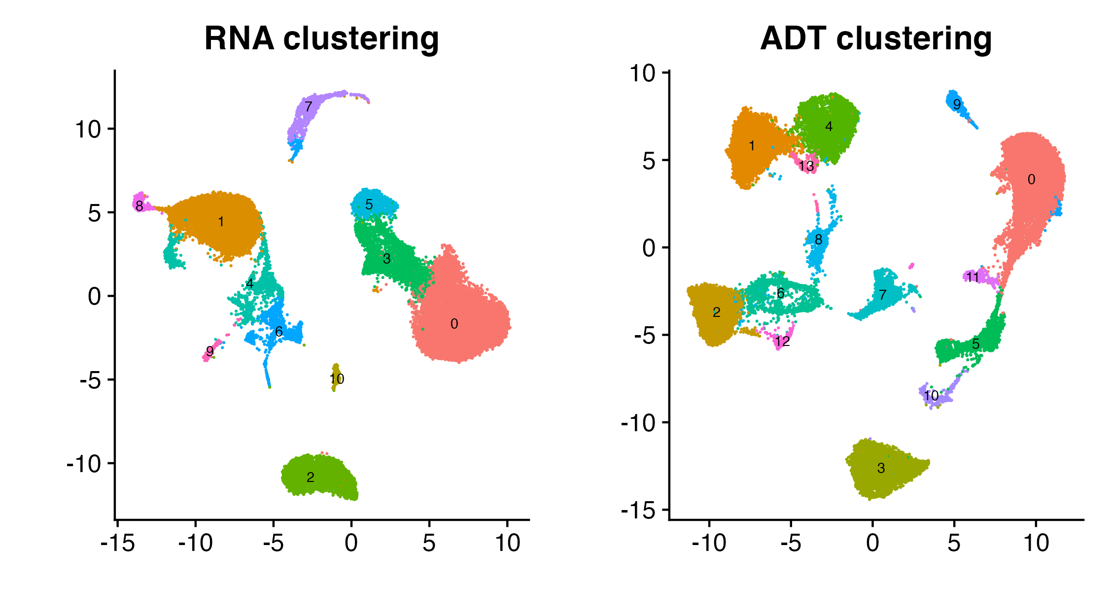
Modality-specific clustering structure
Note: These two clusters are not the same. The colorings in each of the two above plots are not related.
Extracting the relevant matrices
We now extract the relevant matrices for Tilted-CCA. Since Tilted-CCA
is designed not necessarily for single-cell data, we don’t pass the
Seurat object directly into Tilted-CCA. Instead, we extract the relevant
matrices, where the rows are the cells and the columns are various
features (i.e., genes and antibodies). We also remove features that has
negligible empirical standard deviation. (In this tutorial, no genes or
antibodies were removed in this step.) We end up with
mat_1b that has 30,672 cells and 2000 genes, and
mat_2b that has the same 30,672 cells and 25 surface
antibody markers.
Seurat::DefaultAssay(bm) <- "RNA"
mat_1 <- Matrix::t(bm[["RNA"]]@data[Seurat::VariableFeatures(object = bm),])
Seurat::DefaultAssay(bm) <- "ADT"
mat_2 <- Matrix::t(bm[["ADT"]]@data)

mat_1b <- mat_1
sd_vec <- sparseMatrixStats::colSds(mat_1b)
if(any(sd_vec <= 1e-6)){
  mat_1b <- mat_1b[,-which(sd_vec <= 1e-6)]
}

mat_2b <- mat_2
sd_vec <- sparseMatrixStats::colSds(mat_2b)
if(any(sd_vec <= 1e-6)){
  mat_2b <- mat_2b[,-which(sd_vec <= 1e-6)]
}
Running Tilted-CCA
We start Tilted-CCA by first preparing all the low-dimensional
embeddings via tiltedCCA::create_multiSVD. Most of the
boolean arguments are meant to tell our method on whether or not
features are centered and/or scaled (or alternatively, the singular
vectors are centered and/or scaled). We would recommend the boolean
parameters here for any single-cell multiomic data that measures RNA and
antibodies.
set.seed(10)
multiSVD_obj <- tiltedCCA::create_multiSVD(mat_1 = mat_1b, mat_2 = mat_2b,
                                           dims_1 = 1:30, dims_2 = 1:18,
                                           center_1 = T, center_2 = T,
                                           normalize_row = T,
                                           normalize_singular_value = T,
                                           recenter_1 = F, recenter_2 = F,
                                           rescale_1 = F, rescale_2 = F,
                                           scale_1 = T, scale_2 = T,
                                           verbose = 1)
We then pass in the clusterings (one for the RNA, one for the ADT) as
well as form metacells via tiltedCCA::form_metacells. The
metacells help speed up all the later Tilted-CCA calculations. In
general, we recommend using 5000 metacells if the number of cells is
dramatically larger than 5000.
multiSVD_obj <- tiltedCCA::form_metacells(input_obj = multiSVD_obj,
                                          large_clustering_1 = as.factor(bm$RNA_snn_res.0.25),
                                          large_clustering_2 = as.factor(bm$ADT_snn_res.0.25),
                                          num_metacells = 5000,
                                          verbose = 1)
This next step, using tiltedCCA::compute_snns, is
arguably the most subjective step of Tilted-CCA, but nonetheless can
dramatically impact the results if not chosen with care. Here:
-
latent_kdictates how many latent dimensions are extracted from the Laplacian bases of the shared nearest neighbor graphs -
num_neighdictates how many nearest neighbors are used for each cell when constructing the nearest neighbor graphs -
bool_cosinedictates if distance between cells is based on the cosine distance (ifTRUE, i.e., Euclidean distance after normalizing each gene’s low-dimensional embedding to have Euclidean length 1) or Euclidean distance (ifFALSE) -
bool_intersectdictates if an edge is placed between two cells only if each cell is a nearest neighbor of the other cell (ifTRUE) or if an edge is placed between two cells as long as one cell is a nearest neighbor of the other cell (ifFALSE) -
min_degdictates the smallest number of edges for each cell (which is only relevant ifbool_intersect=TRUE), and this value should be a value smaller or equal tonum_neigh
multiSVD_obj <- tiltedCCA::compute_snns(input_obj = multiSVD_obj,
                                        latent_k = 20,
                                        num_neigh = 30,
                                        bool_cosine = T,
                                        bool_intersect = F,
                                        min_deg = 30,
                                        verbose = 2)
Then, we initialize the tilt for all 18 latent dimensions (i.e., the
minimum between the number of latent dimensions in dims_1
and dims_2) via tiltedCCA::tiltedCCA.
multiSVD_obj <- tiltedCCA::tiltedCCA(input_obj = multiSVD_obj,
                                     verbose = 1)
Finally, we fine tune the tilt of each latent dimension. This step can take a while. On a 2020 Macbook Pro (Big Sur, with a Quad-Core Intel Core i7), this step takes around 20 minutes.
multiSVD_obj <- tiltedCCA::fine_tuning(input_obj = multiSVD_obj,
                                       verbose = 1)
After running tiltedCCA:fine_tuning, it is recommended
to save multiSVD_obj since this was the most expensive
calculation (in terms of computation time). The last function call
simply takes the tilts of each latent dimension to compute the full
decomposition of each modality (i.e., cell by feature matrix), four in
total (i.e., a common and distinct for each RNA and ADT). While this
function doesn’t take too much computation time, it greatly expands the
memory size of the multiSVD_obj object.
multiSVD_obj <- tiltedCCA::tiltedCCA_decomposition(input_obj = multiSVD_obj,
                                                   verbose = 1)
Downstream analysis of Tilted-CCA
Congratulations! You have computed the common and distinct embeddings for the single-cell multiomic data. There are various downstream diagnostics you can apply.
Visualizing the common and distinct embeddings
set.seed(10)
bm[["common_tcca"]] <- tiltedCCA::create_SeuratDim(input_obj = multiSVD_obj,
                                                   what = "common",
                                                   aligned_umap_assay = "rna.umap",
                                                   seurat_obj = bm,
                                                   seurat_assay = "RNA",
                                                   verbose = 1)
set.seed(10)
bm[["distinct1_tcca"]] <- tiltedCCA::create_SeuratDim(input_obj = multiSVD_obj,
                                                      what = "distinct_1",
                                                      aligned_umap_assay = "rna.umap",
                                                      seurat_obj = bm,
                                                      seurat_assay = "RNA",
                                                      verbose = 1)
set.seed(10)
bm[["distinct2_tcca"]] <- tiltedCCA::create_SeuratDim(input_obj = multiSVD_obj,
                                                      what = "distinct_2",
                                                      aligned_umap_assay = "rna.umap",
                                                      seurat_obj = bm,
                                                      seurat_assay = "RNA",
                                                      verbose = 1)
We can now plot all three embeddings. Observe how in the common embedding, all the major cell types such as B cells (blue), T cells (mustard, green, and gray) and Monocytes/DC (pink) are separate from one another. This is because both the RNA and ADT modality exhibit these large separation structures. However, because the RNA modality does not cleanly separate the CD8 T-cells from the CD4 T-cells (which only the ADT modality does), there is no apparent separation between these two T-cell sub-types in the common embedding. The RNA distinct embedding displays further separation of the Monocytes/DC, while the ADT distinct embedding displays further separation of the CD8 T-cells from the CD4 T-cells (green and mustard respectively).
p1 <- Seurat::DimPlot(bm,
                      reduction = "common_tcca",
                      group.by = "celltype.l2",
                      cols = col_palette,
                      label = T, repel = T, label.size = 2.5)
p1 <- p1 + Seurat::NoLegend()
p1 <- p1 + ggplot2::ggtitle("Common") + ggplot2::labs(x = "", y = "")
p1 <- p1 + ggplot2::theme(legend.text = ggplot2::element_text(size = 5))

p2 <- Seurat::DimPlot(bm,
                      reduction = "distinct1_tcca",
                      group.by = "celltype.l2",
                      cols = col_palette,
                      label = T, repel = T, label.size = 2.5)
p2 <- p2 + Seurat::NoLegend()
p2 <- p2 + ggplot2::ggtitle("RNA Distinct") + ggplot2::labs(x = "", y = "")
p2 <- p2 + ggplot2::theme(legend.text = ggplot2::element_text(size = 5))

p3 <- Seurat::DimPlot(bm,
                      reduction = "distinct2_tcca",
                      group.by = "celltype.l2",
                      cols = col_palette,
                      label = T, repel = T, label.size = 2.5)
p3 <- p3 + Seurat::NoLegend()
p3 <- p3 + ggplot2::ggtitle("ADT Distinct") + ggplot2::labs(x = "", y = "")
p3 <- p3 + ggplot2::theme(legend.text = ggplot2::element_text(size = 5))

p_all <- cowplot::plot_grid(p1, p2, p3, ncol = 3)
p_all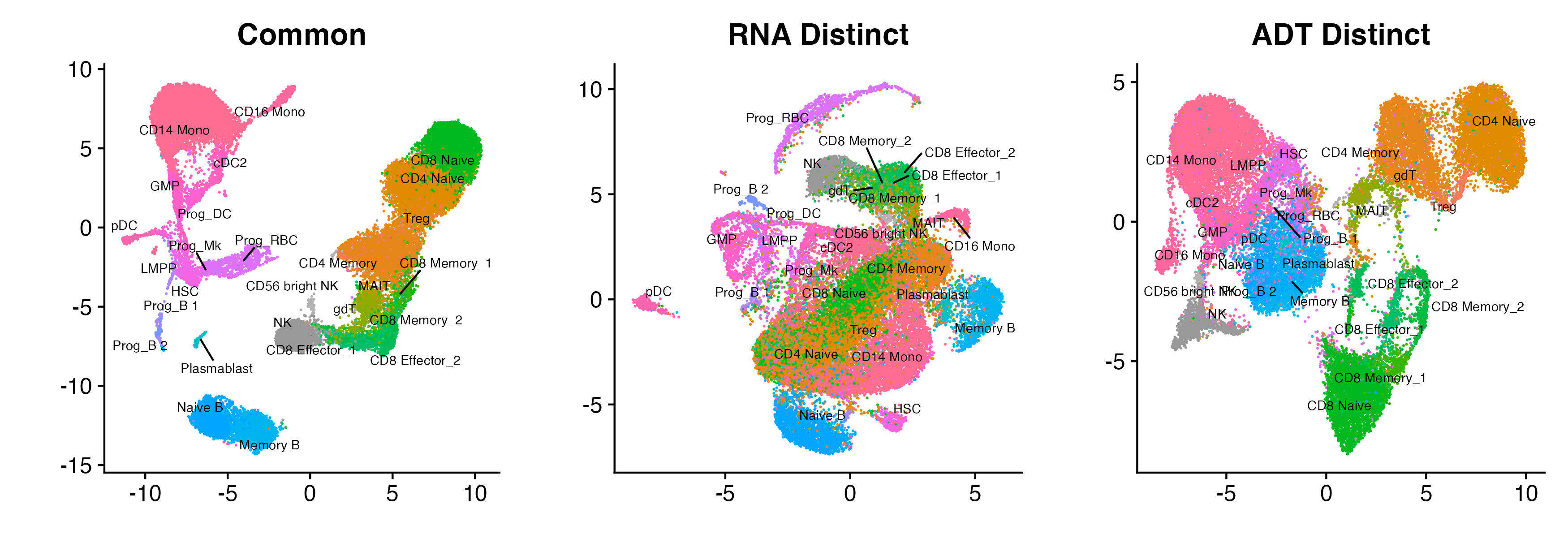
Common, RNA distinct, and ADT distinct embeddings
Assessing how enriched each cell type is in the common or distinct embeddings
Equipped with the common and distinct embeddings, we can more
formally quantify our visual interprations from above. Specifically, we
can compute the percentage of cell types near each cell. If a cell is
“enriched” in a particular embedding (for example, the RNA distinct
embedding), this means that most of the nearest neighbors of that cell
have the same cell type. We perform these calculations using the
tiltedCCA::postprocess_cell_enrichment function. This takes
about 5 minutes.
membership_vec <- factor(bm$celltype.l2)
cell_enrichment_res <- tiltedCCA::postprocess_cell_enrichment(
  input_obj = multiSVD_obj,
  membership_vec = membership_vec,
  max_subsample = 1000,
  verbose = 1
)
We can then visualize these cell-type enrichments. Observe that in
the left plot, the values go from 1 to 0 (along the x-axis), while in
the right plot, the values go from 0 to 1 (along the x-axis). To read
this plot, each cell type is represented as a dot (with color in
col_palette). The higher a cell type is on the y-axis, the
more it means that a cell type’s separation from all other cell types is
supported by both modalities. The more a cell type is to the extremes of
the plot (i.e., a value of 1 on either of the x-axis), the more it means
there is extra information in that modality that separates that cell
type from other cell types that is not reflect in the other modality.
The y-axis value for each cell type is the same in each plot.
tiltedCCA::plot_cell_enrichment(cell_enrichment_res,
                                col_palette = col_palette,
                                cex_axis = 1.25,
                                cex_lab = 1.5,
                                xlab_1 = "RNA Distinct",
                                xlab_2 = "ADT Distinct")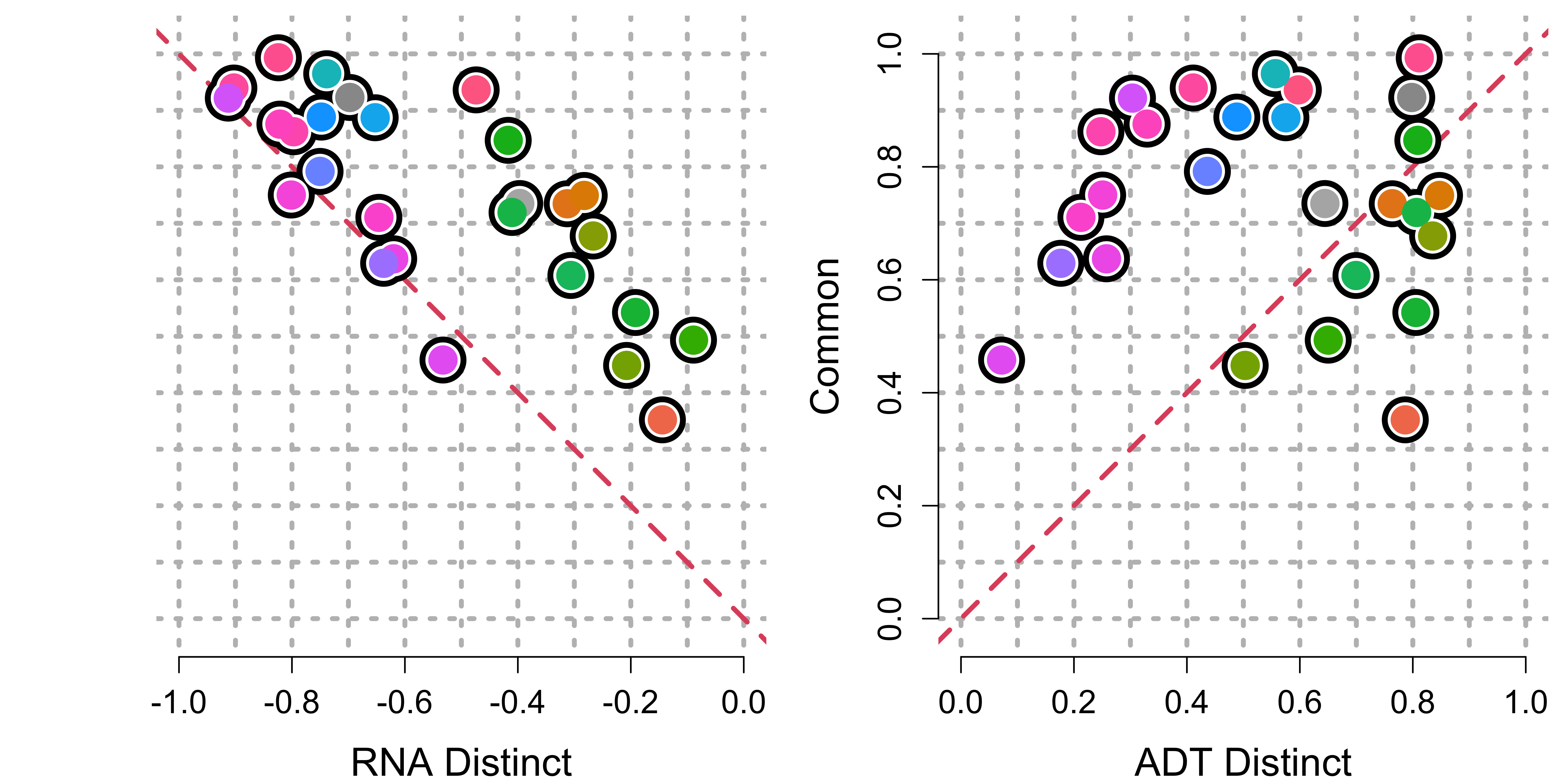
Cell type enrichment of common vs. distinct
Assessing the alignment of each gene with the common embedding
We now strive to assess how aligned each gene is with the common embedding, relative to how “important” the gene is in separating the cell types apart. We run the following code to simplify number of cell types to consider, because in what’s to come, we will be running a differential-expression (DE) test between each pair of cell types.
celltype_l3 <- as.character(bm$celltype.l2)
celltype_l3[celltype_l3 %in% c("NK", "CD56 bright NK")] <- "NK_all"
celltype_l3[celltype_l3 %in% c("MAIT", "gdT")] <- "MAIT-gdT"
celltype_l3[celltype_l3 %in% c("Memory B", "Naive B")] <- "B"
celltype_l3[celltype_l3 %in% c("Prog_B 1", "Prog_B 2")] <- "Prog_B"
celltype_l3[celltype_l3 %in% c("Prog_Mk", "Plasmablast", "LMPP", "Treg")] <- NA
col_palette2 <- c(col_palette,
                  col_palette["NK"],
                  col_palette["MAIT"],
                  col_palette["Memory B"],
                  col_palette["Prog_B 1"])
names(col_palette2) <- c(names(col_palette), "NK_all", "MAIT-gdT", "B", "Prog_B")
Since there are 19 different cell types, there are 171 pairwise comparisons to make. This would be too many comparisons for a short tutorial. Hence, if you do not currently have time to run a multi-hour computation, please run the following line. This subsets the cell types to be only 4.
# RECOMMEND: For a short tutorial, please run this line
keep_celltypes <- c("CD4 Naive", "CD8 Naive", "B", "CD14 Mono")
celltype_l3[!celltype_l3 %in% keep_celltypes] <- NA
As long as celltype_l3 only has 4 cell types, this
following calculation would take only 20 minutes (again, on a 2020
Macbook Pro, Big Sur, with a Quad-Core Intel Core i7). The result is a
vector logpval_vec, which contains the negative log10
p-value for each of the 2000 highly variable genes. Please see the
documentation for tiltedCCA::differential_expression on how
exactly this p-value was derived.
bm$celltype.l3 <- celltype_l3
gene_de_list <- tiltedCCA::differential_expression(seurat_obj = bm,
                                                   assay = "RNA",
                                                   idents = "celltype.l3",
                                                   test_use = "MAST",
                                                   slot = "counts")

logpval_vec <- tiltedCCA::postprocess_depvalue(de_list = gene_de_list,
                                               maximum_output = 300)
The former calculation tells us how “important” a gene is in
separating the cell types apart. We now need to compute how aligned a
gene is with the common embedding. This is what we do with the
tiltedCCA::postprocess_modality_alignment function.
rsquare_vec <- tiltedCCA::postprocess_modality_alignment(input_obj = multiSVD_obj,
                                                         bool_use_denoised = T,
                                                         seurat_obj = bm,
                                                         input_assay = 1,
                                                         seurat_assay = "RNA",
                                                         seurat_slot = "data")
We are almost ready to plot rsquare_vec against
logpval_vec. Before doing so, it’s informative to compute a
few more statistics. Here, gene_color[ord_idx] is a color
vector that will help visually inform us of which genes have a high
sequencing depth.
col_palette_enrichment <- paste0(grDevices::colorRampPalette(c('lightgrey', 'blue'))(100), "33")
gene_breaks <- seq(0, 0.18, length.out = 100)
gene_depth <- Matrix::rowSums(bm[["RNA"]]@counts[names(rsquare_vec),])/n
gene_depth <- log10(gene_depth+1)
gene_color <- sapply(gene_depth, function(x){
  col_palette_enrichment[which.min(abs(gene_breaks - x))]
})
ord_idx <- order(gene_depth, decreasing = F)
Next, we need to focus on a few “marker” genes to display in our
plots. We can use the
tiltedCCA::postprocess_marker_variables for this matter,
since our previous call to
tiltedCCA::differential_expression has already computed all
the pairwise DE tests. We also grab the cell-cycling marker genes from
Seurat.
gene_list <- tiltedCCA::postprocess_marker_variables(de_list)
cycling_genes <- c(cc.genes$s.genes[which(cc.genes$s.genes %in% names(logpval_vec))],
                   cc.genes$g2m.genes[which(cc.genes$g2m.genes %in% names(logpval_vec))])
Finally, we are ready to make the alignment plots. Here, we plot 4 of them. The first shows all the genes, where the genes are colored by the sequencing depth. The next two plots specifically highlight the marker genes for either B cells or CD14 Monocytes. We see that the marker genes are 1) to the right on the x-axis (denoting their very significant p-values, which defines what makes a marker gene) but also 2) very high on the y-axis (denoting that these genes express a signature that is corroborated by both the RNA and ADT modalities). The last plot shows the cell cycling genes, which are 1) in the middle of the x-axis (denoting that these genes don’t differentiate any pair of cell types) and 2) in the middle of the y-axis (denoting that these genes express a signature that is not reflected in the ADT modality).
par(mfrow = c(1,4), mar = c(5,5,5,1))
tiltedCCA::plot_alignment(rsquare_vec = rsquare_vec[ord_idx],
                          logpval_vec = logpval_vec[ord_idx],
                          main = "Human BM (CITE-Seq, RNA+ADT)\nGene differentiability vs. alignment",
                          bool_mark_ymedian = T,
                          col_gene_highlight_border = rgb(255, 205, 87, 255*0.5, maxColorValue = 255),
                          col_points = gene_color[ord_idx],
                          mark_median_xthres = 10,
                          lwd_polygon_bold = 3)

for(i in 1:2){
  tiltedCCA::plot_alignment(rsquare_vec = rsquare_vec,
                            logpval_vec = logpval_vec,
                            main = paste0("Human BM (CITE-Seq, RNA+ADT)\n", names(gene_list)[i], " genes"),
                            col_gene_highlight = col_palette2[names(gene_list)[i]],
                            gene_names = gene_list[[i]],
                            lwd_polygon_bold = 3)
}

tiltedCCA::plot_alignment(rsquare_vec = rsquare_vec,
                          logpval_vec = logpval_vec,
                          main = "Human BM (CITE-Seq, RNA+ADT)\nCell cycling genes",
                          col_gene_highlight = "black",
                          gene_names = cycling_genes,
                          lwd_polygon_bold = 3)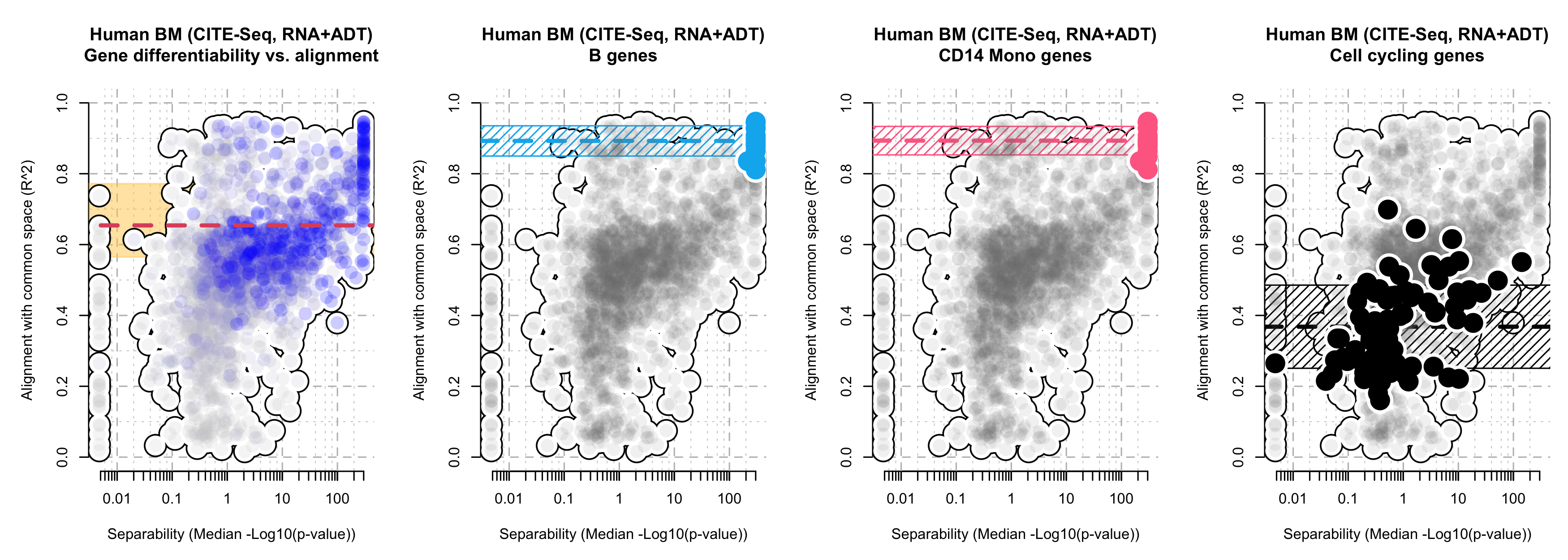
Gene alignment plots, for all genes, or highlight the marker genes for B cells, CD14 Monocytes, or cell cycling