Analysis of human embryo
embryo.RmdWe go through how to analyze single-cell multiomic data in this vignette (RNA and ATAC). We focus on a 10x Multiome data from Trevino et al., Cell, 2021, which can be downloaded directly from their GitHub. Relevant citation:
Trevino, A. E., Müller, F., Andersen, J., Sundaram, L., Kathiria, A., Shcherbina, A., ... & Greenleaf, W. J. (2021). Chromatin and gene-regulatory dynamics of the developing human cerebral cortex at single-cell resolution. Cell, 184(19), 5053-5069.Preliminary analysis
We will work from a simplified preprocessed version of the data, already compiled as a Seurat object, which you can download from https://www.dropbox.com/s/gh2om9eb5edgi14/10x_trevino_simplified.RData (about 0.34 Gigabytes in size). To make the data more portable, important biological information (not relevant to our Tilted-CCA analysis in this vignette) is discarded. Please refer to our original preprocessing script to see how to preprocess the data with the full biological information.
Loading the data
After downloading the file from the Dropbox link, load it into your R session.
load("/Users/kevinlin/Library/CloudStorage/Dropbox/Collaboration-and-People/Nancy/multiomeFate/out/vignettes/10x_trevino_simplified.RData")
seurat_obj
#> An object of class Seurat
#> 271643 features across 6158 samples within 2 assays
#> Active assay: SCT (2027 features, 2027 variable features)
#>  1 layer present: data
#>  1 other assay present: ATAC
This data has 6361 cells with 2027 genes and 269616 peaks.
If we look at metadata, we see that the cell types are also provided (6 cell types in total).
table(seurat_obj$celltype)
#>  Cyc. Prog.      GluN2      GluN3      GluN4      GluN5 nIPC/GluN1         RG
#>         341       1546        798        459        223       2348        646
We need now preprocess the data using a typical procedure. While the data provided in this vignette is already normalized (RNA via SCTransform, and ATAC via the typical Signac pipeline), we need to compute the embeddings.
set.seed(10)
Seurat::DefaultAssay(seurat_obj) <- "SCT"
seurat_obj <- Seurat::ScaleData(seurat_obj)
seurat_obj <- Seurat::RunPCA(seurat_obj,
                             verbose = FALSE)
seurat_obj <- Seurat::RunUMAP(seurat_obj,
                              dims = 1:50,
                              reduction.name = "umap.rna",
                              reduction.key = "rnaUMAP_")

set.seed(10)
seurat_obj <-  Signac::RunSVD(seurat_obj)
seurat_obj <- Seurat::RunUMAP(seurat_obj,
                              reduction = "lsi",
                              dims = 2:50,
                              reduction.name = "umap.atac",
                              reduction.key = "atacUMAP_")

seurat_obj <- tiltedCCA::rotate_seurat_embeddings(
  seurat_obj = seurat_obj,
  source_embedding = "umap.rna",
  target_embedding = "umap.atac"
)
col_palette <- c(
  "Cyc. Prog." = rgb(213, 163, 98, maxColorValue = 255),
  "GluN2" = rgb(122, 179, 232, maxColorValue = 255),
  "GluN3"= rgb(174, 198, 235, maxColorValue = 255),
  "GluN4" = rgb(217, 227, 132, maxColorValue = 255),
  "GluN5" = rgb(127, 175, 123, maxColorValue = 255),
  "nIPC/GluN1" = rgb(114, 169, 158, maxColorValue = 255),
  "RG" = rgb(197, 125, 95, maxColorValue = 255)
)


p1 <- Seurat::DimPlot(seurat_obj,
                      reduction = "umap.rna",
                      group.by = "celltype",
                      cols = col_palette,
                      label = T, repel = T, label.size = 2.5)
p1 <- p1 + Seurat::NoLegend()
p1 <- p1 + ggplot2::ggtitle("RNA") + ggplot2::labs(x = "", y = "")
p1 <- p1 + ggplot2::theme(legend.text = ggplot2::element_text(size = 5))

p2 <- Seurat::DimPlot(seurat_obj,
                      reduction = "umap.atac",
                      group.by = "celltype",
                      cols = col_palette,
                      label = T, repel = T, label.size = 2.5)
p2 <- p2 + Seurat::NoLegend()
p2 <- p2 + ggplot2::ggtitle("ATAC") + ggplot2::labs(x = "", y = "")
p2 <- p2 + ggplot2::theme(legend.text = ggplot2::element_text(size = 5))

p_all <- cowplot::plot_grid(p1, p2, ncol = 2)
p_all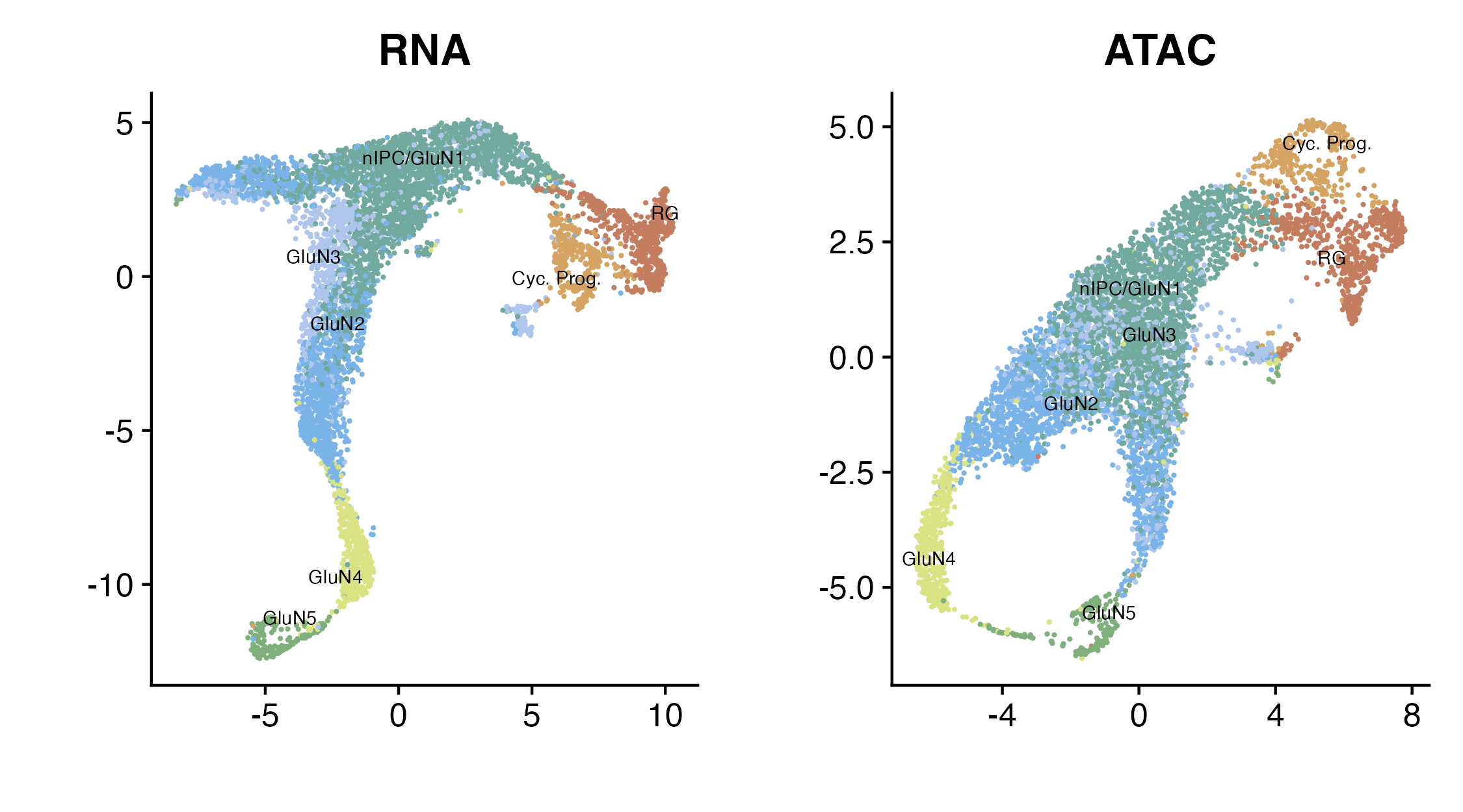
UMAPs of the RNA modality (left) and ATAC modality (right)
Running Tilted-CCA
We are now ready to run Tilted-CCA.
Extracting the relevant matrices
We now extract the relevant matrices for Tilted-CCA. Since Tilted-CCA
is designed not necessarily for single-cell data, we don’t pass the
Seurat object directly into Tilted-CCA. Instead, we extract the relevant
matrices, where the rows are the cells and the columns are various
features (i.e., genes and accessible chromatin regions). We also remove
features that has negligible empirical standard deviation. (In this
tutorial, no genes or accessible chromatin region were removed in this
step.) We end up with mat_1b that has 30,672 cells and 2000
genes, and mat_2b that has the same 30,672 cells and
269,616 accessible chromatin regions.
Seurat::DefaultAssay(seurat_obj) <- "SCT"
mat_1 <- Matrix::t(seurat_obj[["SCT"]]@data)
Seurat::DefaultAssay(seurat_obj) <- "ATAC"
mat_2 <- Matrix::t(seurat_obj[["ATAC"]]@data)

mat_1b <- mat_1
sd_vec <- sparseMatrixStats::colSds(mat_1b)
if(any(sd_vec <= 1e-6)){
  mat_1b <- mat_1b[,-which(sd_vec <= 1e-6)]
}

mat_2b <- mat_2
sd_vec <- sparseMatrixStats::colSds(mat_2b)
if(any(sd_vec <= 1e-6)){
  mat_2b <- mat_2b[,-which(sd_vec <= 1e-6)]
}
Running Tilted-CCA
We start Tilted-CCA by first preparing all the low-dimensional
embeddings via tiltedCCA::create_multiSVD. Most of the
boolean arguments are meant to tell our method on whether or not
features are centered and/or scaled (or alternatively, the singular
vectors are centered and/or scaled). We would recommend the boolean
parameters here for any single-cell multiomic data that measures RNA and
chromatin regions.
set.seed(10)
multiSVD_obj <- tiltedCCA::create_multiSVD(mat_1 = mat_1b, mat_2 = mat_2b,
                                           dims_1 = 1:50, dims_2 = 2:50,
                                           center_1 = T, center_2 = F,
                                           normalize_row = T,
                                           normalize_singular_value = T,
                                           recenter_1 = F, recenter_2 = T,
                                           rescale_1 = F, rescale_2 = T,
                                           scale_1 = T, scale_2 = F,
                                           verbose = 1)
We then go to the next step of
tiltedCCA::form_metacells. To make this tutorial be more
portable, we downscale the calculation to only involve 100 metacells.
However, since the UMAPs display a continuous transition of cell states,
we do not need to pass any hard clustering information.
multiSVD_obj <- tiltedCCA::form_metacells(input_obj = multiSVD_obj,
                                          large_clustering_1 = NULL,
                                          large_clustering_2 = NULL,
                                          num_metacells = 100,
                                          verbose = 1)
This next step, using tiltedCCA::compute_snns, is
arguably the most subjective step of Tilted-CCA, but nonetheless can
dramatically impact the results if not chosen with care. Here:
-
latent_kdictates how many latent dimensions are extracted from the Laplacian bases of the shared nearest neighbor graphs -
num_neighdictates how many nearest neighbors are used for each cell when constructing the nearest neighbor graphs -
bool_cosinedictates if distance between cells is based on the cosine distance (ifTRUE, i.e., Euclidean distance after normalizing each gene’s low-dimensional embedding to have Euclidean length 1) or Euclidean distance (ifFALSE) -
bool_intersectdictates if an edge is placed between two cells only if each cell is a nearest neighbor of the other cell (ifTRUE) or if an edge is placed between two cells as long as one cell is a nearest neighbor of the other cell (ifFALSE) -
min_degdictates the smallest number of edges for each cell (which is only relevant ifbool_intersect=TRUE), and this value should be a value smaller or equal tonum_neigh
multiSVD_obj <- tiltedCCA::compute_snns(input_obj = multiSVD_obj,
                                        latent_k = 20,
                                        num_neigh = 15,
                                        bool_cosine = T,
                                        bool_intersect = F,
                                        min_deg = 15,
                                        verbose = 1)
Then, we initialize the tilt for all 49 latent dimensions (i.e., the
minimum between the number of latent dimensions in dims_1
and dims_2) via tiltedCCA::tiltedCCA.
multiSVD_obj2 <- tiltedCCA::tiltedCCA(input_obj = multiSVD_obj,
                                      verbose = 1)
Finally, we fine tune the tilt of each latent dimension. This step can take a while. On a 2023 Macbook Pro (Sonoma, Apple M2 Max with 32 Gb of memory), this step takes around 20 minutes.
multiSVD_obj2 <- tiltedCCA::fine_tuning(input_obj = multiSVD_obj2,
                                        verbose = 1)
Results of fine tuning
The tiltedCCA::fine_tuning essentially sets the
appropriate tilts per latent dimension, stored in
multiSVD_obj$tcca_obj$tilt_perc. If you want to directly,
you can directly set the desired tilts using the
fix_tilt_perc argument in
tiltedCCA::fine_tuning. For example, we can run the
following code:
desired_tilt <- c(0.65, 0.85, 0.55, 1.00, 1.00, 0.95,
                  1.00, 1.00, 1.00, 1.00, 1.00, 1.00,
                  0.40, 0.10, 0.70, 0.15, 0.75, 0.00,
                  0.00, 0.45, 0.15, 0.05, 0.80, 0.95,
                  0.65, 0.40, 0.45, 0.40, 0.75, 1.00,
                  0.80, 0.10, 0.00, 0.30, 0.65, 0.05,
                  0.65, 0.85, 0.35, 1.00, 0.85, 0.25,
                  0.90, 0.30, 0.40, 0.95, 0.30, 0.55,
                  0.65)
multiSVD_obj3 <- tiltedCCA::tiltedCCA(input_obj = multiSVD_obj,
                                      fix_tilt_perc = desired_tilt,
                                      verbose = 1)
We can then use multiSVD_obj3 for the rest of the
tutorial, instead of multiSVD_obj2.
After running tiltedCCA::fine_tuning, it is recommended
to save multiSVD_obj2 since this was the most expensive
calculation (in terms of computation time). The last function call
simply takes the tilts of each latent dimension to compute the full
decomposition of each modality (i.e., cell by feature matrix), four in
total (i.e., a common and distinct for each RNA and ADT). While this
function doesn’t take too much computation time, it greatly expands the
memory size of the multiSVD_obj2 object.
multiSVD_obj2 <- tiltedCCA::tiltedCCA_decomposition(input_obj = multiSVD_obj2,
                                                    verbose = 1,
                                                    bool_modality_1_full = T,
                                                    bool_modality_2_full = F)
Downstream analysis of Tilted-CCA
Congratulations! You have computed the common and distinct embeddings for the single-cell multiomic data. There are various downstream diagnostics you can apply.
Visualizing the common and distinct embeddings
set.seed(10)
seurat_obj[["common_tcca"]] <- tiltedCCA::create_SeuratDim(input_obj = multiSVD_obj2,
                                                           what = "common",
                                                           aligned_umap_assay = "umap.rna",
                                                           seurat_obj = seurat_obj,
                                                           seurat_assay = "SCT",
                                                           verbose = 1)
set.seed(10)
seurat_obj[["distinct1_tcca"]] <- tiltedCCA::create_SeuratDim(input_obj = multiSVD_obj2,
                                                              what = "distinct_1",
                                                              aligned_umap_assay = "umap.rna",
                                                              seurat_obj = seurat_obj,
                                                              seurat_assay = "SCT",
                                                              verbose = 1)
set.seed(10)
seurat_obj[["distinct2_tcca"]] <- tiltedCCA::create_SeuratDim(input_obj = multiSVD_obj2,
                                                              what = "distinct_2",
                                                              aligned_umap_assay = "umap.rna",
                                                              seurat_obj = seurat_obj,
                                                              seurat_assay = "SCT",
                                                              verbose = 1)
p1 <- Seurat::DimPlot(seurat_obj,
                      reduction = "common_tcca",
                      group.by = "celltype",
                      cols = col_palette,
                      label = T, repel = T, label.size = 2.5)
p1 <- p1 + Seurat::NoLegend()
p1 <- p1 + ggplot2::ggtitle("Common") + ggplot2::labs(x = "", y = "")
p1 <- p1 + ggplot2::theme(legend.text = ggplot2::element_text(size = 5))

p2 <- Seurat::DimPlot(seurat_obj,
                      reduction = "distinct1_tcca",
                      group.by = "celltype",
                      cols = col_palette,
                      label = T, repel = T, label.size = 2.5)
p2 <- p2 + Seurat::NoLegend()
p2 <- p2 + ggplot2::ggtitle("RNA Distinct") + ggplot2::labs(x = "", y = "")
p2 <- p2 + ggplot2::theme(legend.text = ggplot2::element_text(size = 5))

p3 <- Seurat::DimPlot(seurat_obj,
                      reduction = "distinct2_tcca",
                      group.by = "celltype",
                      cols = col_palette,
                      label = T, repel = T, label.size = 2.5)
p3 <- p3 + Seurat::NoLegend()
p3 <- p3 + ggplot2::ggtitle("ATAC Distinct") + ggplot2::labs(x = "", y = "")
p3 <- p3 + ggplot2::theme(legend.text = ggplot2::element_text(size = 5))

p_all <- cowplot::plot_grid(p1, p2, p3, ncol = 3)
p_all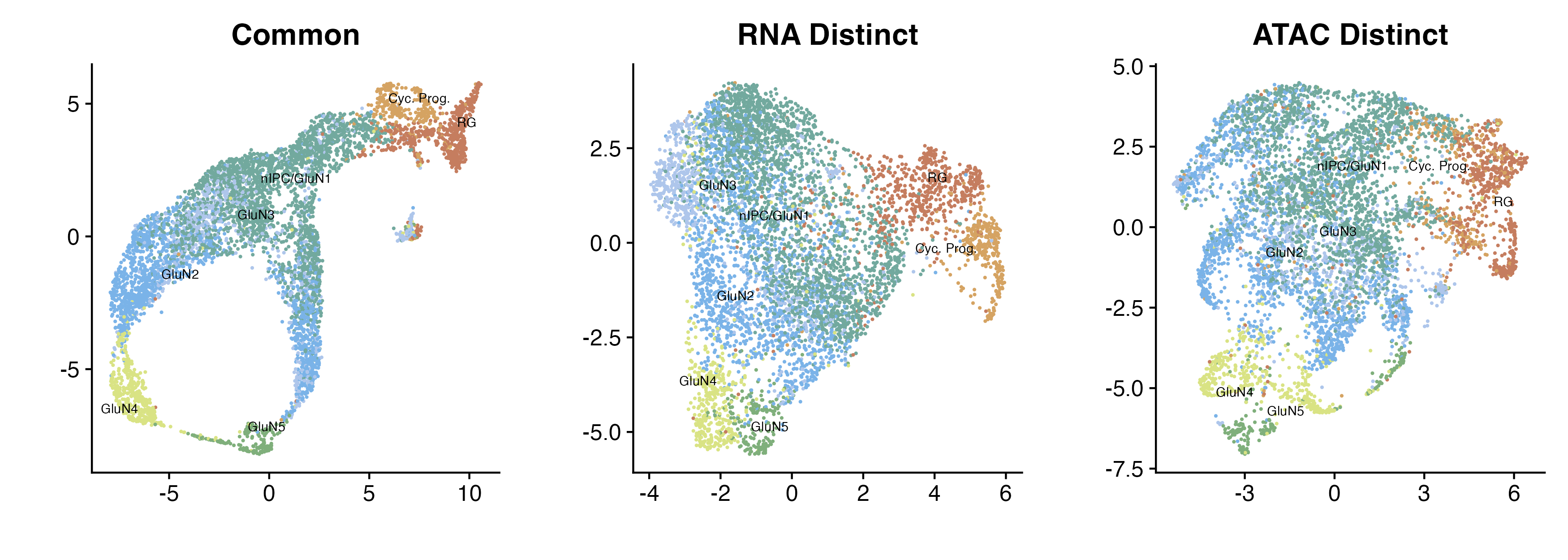
Common, RNA distinct, and ATAC distinct embeddings
Compute sychrony scores
We can now compute the synchrony score between the two modalities, where each cell gets a score. If the score is close to 1, it means that for this cell, the ATAC profile is “similar” to that for the RNA profile, where “similar” here (conceptually) means that the cell has similar nearest neighbors in ATAC as those in the RNA profile. Typically, we interpret this cell as in the steady state, which means it is not in the process of differentiating (i.e., one modality is changing before another). In contrast, if the score is close to 0, it means that for this cell, the two modalities contain vastly different information. Typically, we interpret this cell as having one modality experiencing a change that is not yet reflected in the other modality. The specific calculation for the synchrony score relies on the low-dimension embeddings learned by Tilted-CCA.
synchrony_score <- tiltedCCA::compute_synchrony(input_obj = multiSVD_obj2)

seurat_obj$synchrony <- synchrony_score[Seurat::Cells(seurat_obj),"synchrony_rescaled"]

p1 <- Seurat::FeaturePlot(seurat_obj,
                    reduction = "common_tcca",
                    feature = "synchrony",
                    cols = c("forestgreen", "yellow"))
p1 <- p1 + ggplot2::ggtitle("Synchrony score") + ggplot2::labs(x = "Common TCCA 1", y = "Common TCCA 2")
p1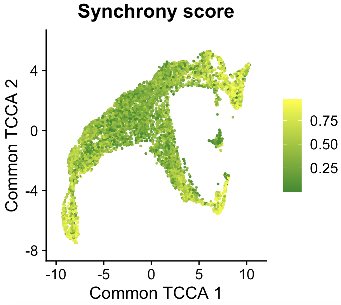
Synchrony score
Comparing this plot to the “Common, RNA distinct, and ATAC distinct embeddings” plot shows that the terminal cells (radial glia, glutamatergic 4 and glutamatergic 5) have high synchrony scores, meaning these cells are in a steady state. In contrast, the cells undergoing differentiation (glutamatergic 1 and glutamatergic 3) have low synchrony scores. This demonstrates the utility of the synchrony score. Importantly, the calculation of the synchrony scores does not require any pseudotime or trajectories – it’s entirely based on the Tilted-CCA embeddings, which makes this method appealing even for complex differentiation systems with many branching trajectories.