Tilted-CCA Overview
tiltedCCA.RmdPurpose
The simulations here are meant to be portable, toy-examples of Tilted-CCA, with the intent to demonstrate that an installation of Tilted-CCA was successful as well as to demonstrate how it differs from the methods that seek to find the “union of information”.
A successful installation of tiltedCCA is required for
this. See the last section of this README of all the system/package
dependencies used when creating these simulations. Both simulations
should complete in less than 2 minutes.
Overview
Broadly speaking, Tilted-CCA is a pipeline of 6 different function
calls. The procedure starts by assuming there are two data matrices,
mat_1 and mat_2, (either matrix
or dgCMatrix) with the same number of rows (i.e., the same
cells), but possibly different features. We advise making sure each
row/column of either matrix has non-zero variance prior to using this
pipeline.
-
Step 1 (Initializing low-rank representation of each
modality,
create_multiSVD): We compute the leading PCs of each modality here. There can be a different number of latent dimensions for each modality. Here, the additional parameters dictate how to compute the leading PCs (for example, should the features be scaled/center before or after the computing the PCs? Which PCs should be used downstream? This would be useful since for ATAC data, it is common to not use the first leading PC.)
This typically looks like the following.
multiSVD_obj <- tiltedCCA::create_multiSVD(mat_1 = mat_1, mat_2 = mat_2,
                                           dims_1 = 1:2, dims_2 = 1:2,
                                           center_1 = F, center_2 = F,
                                           normalize_row = T,
                                           normalize_singular_value = F,
                                           recenter_1 = F, recenter_2 = F,
                                           rescale_1 = F, rescale_2 = F,
                                           scale_1 = F, scale_2 = F)
The output of this step is a multiSVD object, which will
continually be updated as we feed it as input and get an updated object
after each of the following function calls. It currently has elements
svd_1, svd_2, default_assay, and
param.
-
Step 2 (Passing helping information,
form_metacells): We pass (optional) large clustering structure or meta-cells here. The former is designed to help aid Tilted-CCA assess what the “intersection of information” is, and the latter is designed for handling large datasets with more than 10,000 cells. If no large structuring structure is needed, the practitioner can simply pass inlarge_clustering_1=NULLandlarge_clustering_2=NULL. If no meta-cells are needed, the practitioner can simply pass innum_metacells=NULL.
This typically looks like the following.
multiSVD_obj <- tiltedCCA::form_metacells(input_obj = multiSVD_obj,
                                          large_clustering_1 = clustering_1,
                                          large_clustering_2 = clustering_2,
                                          num_metacells = NULL)
The updated multiSVD object will now have an additional
element: metacell_obj.
-
Step 3 (Creating shared nearest neighbor (SNN) graphs,
compute_snns): We compute the SNN graphs for both modalities and the target common manifold (computed based on both modality’s SNN graph). These graphs dictate how Tilted-CCA represents the information in each modality, and each node of the graph represents a cell/meta-cell. Here, the additional parameters dictate the specific details on how these graphs are constructed. The two important parameterslatent_k(i.e., the dimensionality of the graph Laplacian eigenbases, which is used when optimizing the tilt) andnum_neigh(i.e., the number of neighbors for each cell in either modality).
This typically looks like the following.
multiSVD_obj <- tiltedCCA::compute_snns(input_obj = multiSVD_obj,
                                        latent_k = 2,
                                        num_neigh = 10,
                                        bool_cosine = T,
                                        bool_intersect = T,
                                        min_deg = 1)
The updated multiSVD object will now have additional
elements: snn_list and laplacian_list.
-
Step 4 (Initializing Tilted-CCA,
tiltedCCA): We compute the CCA between both modalities and initialize the tilt across all latent dimensions to a particular value. Recall that CCA’s solution can be directly computed using the PC’s from each modality. If there are different number of latent dimensions for each modality, Tilted-CCA will have a latent dimensionality (i.e., via CCA) equal to the smaller of the two.
multiSVD_obj <- tiltedCCA::tiltedCCA(input_obj = multiSVD_obj)The updated multiSVD object will now have additional
elements: cca_obj and tcca_obj.
-
Step 5 (Tuning the tilt across each latent dimension,
fine_tuning): We tune the tilt across each latent dimension. This is the main computational bottleneck of Tilted-CCA, as an optimization is performed cyclically (i.e., the tilt for each latent dimension is updated in sequence, with a few epochs cycling through all latent dimensions).
multiSVD_obj <- tiltedCCA::fine_tuning(input_obj = multiSVD_obj)There is no new obvious element added to multiSVD, but
the representation of the common and distinct embeddings is updated upon
this function’s completion. For example,
multiSVD_obj$tcca_obj$tilt_perc now is a vector, denoting
the tilt of the common vector for each latent dimension.
-
Step 6 (Completing the decomposition,
tiltedCCA_decomposition): Given the tilts of common vectors across all latent dimensions, we now recover the full cell-by-feature decomposition of each modality. Here, the additional parameters dictate whether you want the decompositions to be cell-by-feature or cell-by-PC. The latter is desirable especially if you are analyzing ATAC data, where the cell-by-feature would be a dense matrix with many hundred-of-thousand features (which would be too memory intensive).
multiSVD_obj <- tiltedCCA::tiltedCCA_decomposition(multiSVD_obj)The updated multiSVD object will now have additional
elements: common_mat_1 and distint_mat_1 (or
common_dimred_1 and distinct_dimred_1 if
bool_modality_1_full=F) and common_mat_2 and
distint_mat_2 (or common_dimred_2 and
distinct_dimred_2 if
bool_modality_2_full=F)
Simulation 1: Modality 1 separates cells into 3 clusters, and Modality 2 does not
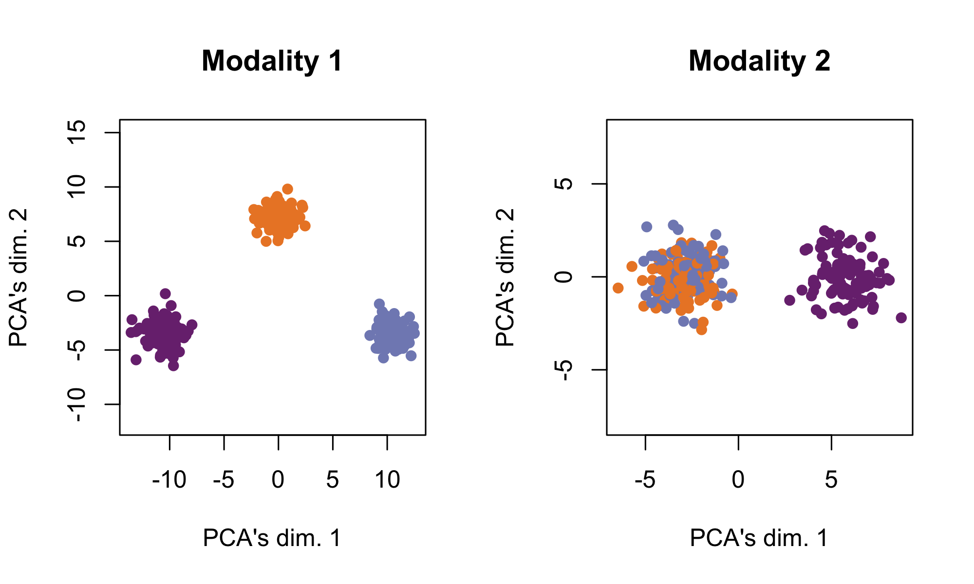
See https://github.com/linnykos/tiltedCCA_analysis/blob/master/simulation/ppt_examples/toy-simulation.R for this simulation. In this simulation, there are 300 cells across two modalities of 10 features each. Modality 1 has a “high” amount of distinct information – it separates the 300 cells into 3 obvious clusters. Modality 2 has a “low” amount of distinct information – all 300 cells are in one amorphous ball.
The following shows each modality based on their leading 2 PCs respectively, where the cells are colored by the true cell-types.
simulation1_data
The following shows Tilted-CCA’s common (i.e., shared axes of variation between both modalities) and distinct (i.e., axes of variation unique to a modality, after the common axes have been accounted for) axes of variation, where the cells are colored by the true cell-types. Here, observe that the common embedding does not really contain information to separate the cell-types – this is desirable, as all the cell-type separation information are unique to Modality 1 (hence, appearing in the Modality 1’s distinct embedding). The common embedding demonstrates the “intersection of information.”
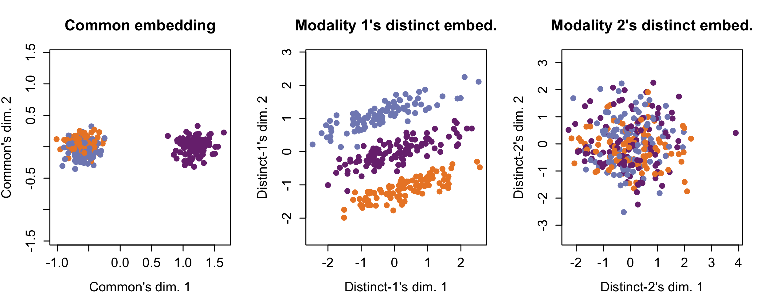
simulation1_tcca
In contrast with Tilted-CCA’s “intersection of information,” we demonstrate Consensus PCA, which is a prototypical method illustrating the “union of information” where a low-dimensional embedding is constructed for multimodal data by combining the leading axes of variation from each modality. These embeddings are useful to visualize the “best of both worlds” (i.e., having cell-type separation that best combines both modalities), but is not useful for to understand the shared and distinct signals between the two modalities. Here, observe that the three cell-types are clearly separated by Consensus PCA.
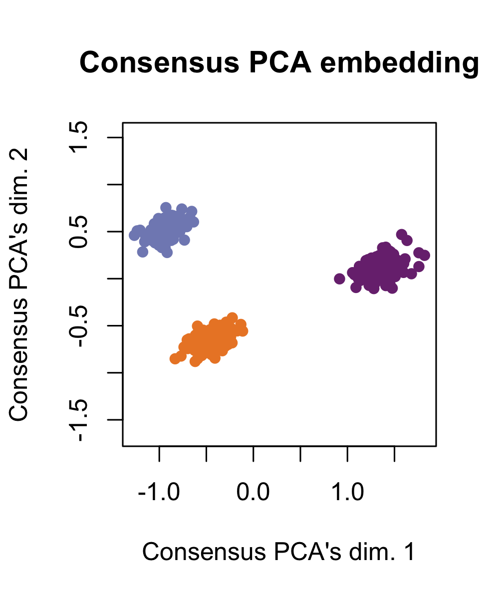
simulation1_consensuspca
Simulation 2: Both modalities separate the 5 cell-types into 3 clusters in different ways
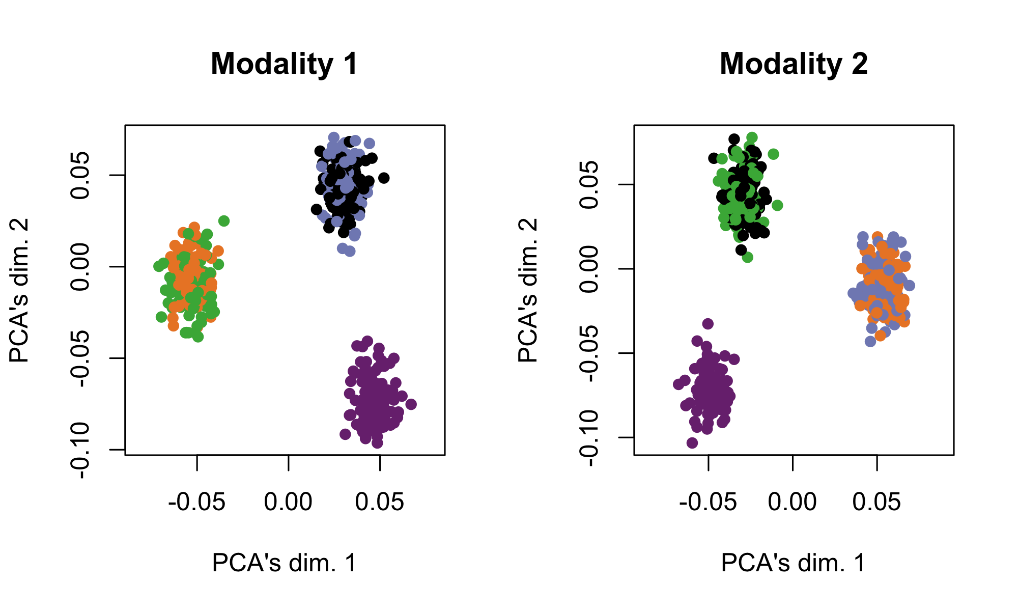
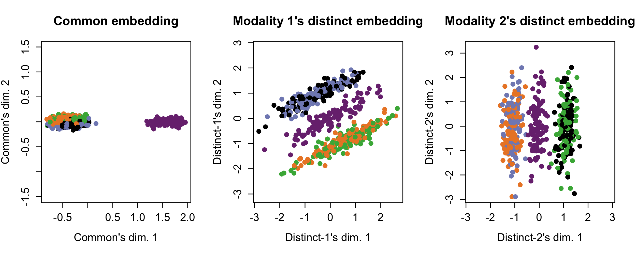
See https://github.com/linnykos/tiltedCCA_analysis/blob/master/simulation/simulation_2.R for this simulation. In this simulation, there are 500 cells across two modalities of 10 features each. There are 5 true cell-types, but each modality can only differentiate these cell-types into 3 clusters. Modality 1 separates the cyan cells from the red+black cells from the green+blue cells, while Modality 2 separates the cyan cells from the red+blue cells from the green+black cells.
The following shows each modality based on their leading 2 PCs respectively, where the cells are colored by the true cell-types.
simulation2_data
The following shows Tilted-CCA’s common (demonstrating the “intersection of information”) and distinct axes of variation, where the cells are colored by the true cell-types. Here, observe that the common embedding shows the information that both modalities agree upon – the cyan cells are separable from all other cell-types. The distinct information then illustrates what is distinct for each modality: Modality 1 separates the cyan cells from the red+black cells from the green+blue cells, while Modality 2 separates the cyan cells from the red+blue cells from the green+black cells.
simulation2_tcca
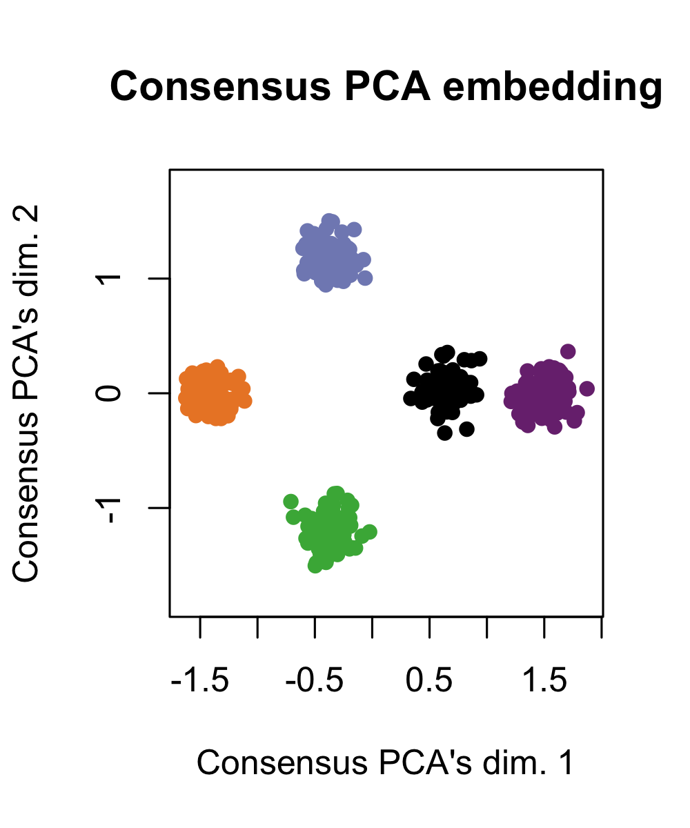
Consensus PCA for this data cleanly separates all five cell-types. Again, quantifying “union of information” is a useful and complementary perspective to what Tilted-CCA does. The “union” gives perspective on what axes of variation are contained across both modalities, while Tilted-CCA’s common embeddings gives perspective on what axes of variation are shared between both modalities.
simulation2_consensuspca
Setup
The following shows the suggested package versions that the developer (GitHub username: linnykos) used when developing the Tilted-CCA package.
> devtools::session_info()
─ Session info ─────────────────────────────────────────────────────
setting  value
version  R version 4.1.2 (2021-11-01)
os       Red Hat Enterprise Linux
system   x86_64, linux-gnu
ui       X11
language (EN)
collate  en_US.UTF-8
ctype    en_US.UTF-8
tz       America/New_York
date     2022-10-04
pandoc   1.12.3.1 @ /usr/bin/pandoc

─ Packages ────────────────────────
package           * version   date (UTC) lib source
cachem        1.0.6      2021-08-19 [1] CRAN (R 4.1.2)
callr         3.7.1      2022-07-13 [1] CRAN (R 4.1.2)
cli           3.3.0      2022-04-25 [1] CRAN (R 4.1.2)
crayon        1.5.1      2022-03-26 [1] CRAN (R 4.1.2)
devtools      2.4.4      2022-07-20 [1] CRAN (R 4.1.2)
digest        0.6.29     2021-12-01 [1] CRAN (R 4.1.2)
ellipsis      0.3.2      2021-04-29 [1] CRAN (R 4.1.2)
fastmap       1.1.0      2021-01-25 [1] CRAN (R 4.1.2)
fs            1.5.2      2021-12-08 [1] CRAN (R 4.1.2)
glue          1.6.2      2022-02-24 [1] CRAN (R 4.1.2)
htmltools     0.5.3      2022-07-18 [1] CRAN (R 4.1.2)
htmlwidgets   1.5.4      2021-09-08 [1] CRAN (R 4.1.2)
httpuv        1.6.5      2022-01-05 [1] CRAN (R 4.1.2)
later         1.3.0      2021-08-18 [1] CRAN (R 4.1.2)
lifecycle     1.0.1      2021-09-24 [1] CRAN (R 4.1.2)
magrittr      2.0.3      2022-03-30 [1] CRAN (R 4.1.2)
memoise       2.0.1      2021-11-26 [1] CRAN (R 4.1.2)
mime          0.12       2021-09-28 [1] CRAN (R 4.1.2)
miniUI        0.1.1.1    2018-05-18 [1] CRAN (R 4.1.2)
pkgbuild      1.3.1      2021-12-20 [1] CRAN (R 4.1.2)
pkgload       1.3.0      2022-06-27 [1] CRAN (R 4.1.2)
prettyunits   1.1.1      2020-01-24 [1] CRAN (R 4.1.2)
processx      3.7.0      2022-07-07 [1] CRAN (R 4.1.2)
profvis       0.3.7      2020-11-02 [1] CRAN (R 4.1.2)
promises      1.2.0.1    2021-02-11 [1] CRAN (R 4.1.2)
ps            1.7.0      2022-04-23 [1] CRAN (R 4.1.2)
purrr         0.3.4      2020-04-17 [1] CRAN (R 4.1.2)
R6            2.5.1      2021-08-19 [1] CRAN (R 4.1.2)
Rcpp          1.0.9      2022-07-08 [1] CRAN (R 4.1.2)
remotes       2.4.2      2021-11-30 [1] CRAN (R 4.1.2)
rlang         1.0.4      2022-07-12 [1] CRAN (R 4.1.2)
sessioninfo   1.2.2      2021-12-06 [1] CRAN (R 4.1.2)
shiny         1.7.2      2022-07-19 [1] CRAN (R 4.1.2)
stringi       1.7.8      2022-07-11 [1] CRAN (R 4.1.2)
stringr       1.4.0      2019-02-10 [1] CRAN (R 4.1.2)
tiltedCCA   * 1.0.0.001  2022-09-06 [1] local
urlchecker    1.0.1      2021-11-30 [1] CRAN (R 4.1.2)
usethis       2.1.6      2022-05-25 [1] CRAN (R 4.1.2)
xtable        1.8-4      2019-04-21 [1] CRAN (R 4.1.2)