2 Introduction
Why study cell biology in public health?
2.1 Why study cell biology in public health?
2.1.1 What are “omics”?
The term “omics” refers to a broad field of biology aimed at the comprehensive characterisation and quantification of biological molecules that translate into the structure, function, and dynamics of an organism. At its core, “omics” encapsulates the idea of studying biological systems at a global scale rather than focusing on individual components. This includes genomics (DNA), transcriptomics (RNA), proteomics (proteins), epigenomics, metabolomics (metabolites), and more. Each of these fields leverages high-throughput technologies to generate massive datasets that capture complex interactions within cells, tissues, or organisms.
The rise of “omics” has revolutionised biology by enabling researchers to ask holistic questions such as how different genes, proteins, or metabolites interact in health and disease. It emphasises understanding systems as interconnected networks rather than isolated elements. This systems-level approach is particularly powerful in identifying biomarkers, understanding disease mechanisms, and tailoring precision-medicine strategies. In public health, “omics” provides tools to bridge molecular discoveries with population-level outcomes, offering new opportunities to tackle complex health challenges.
2.1.2 Some examples of a “cell-biology” question
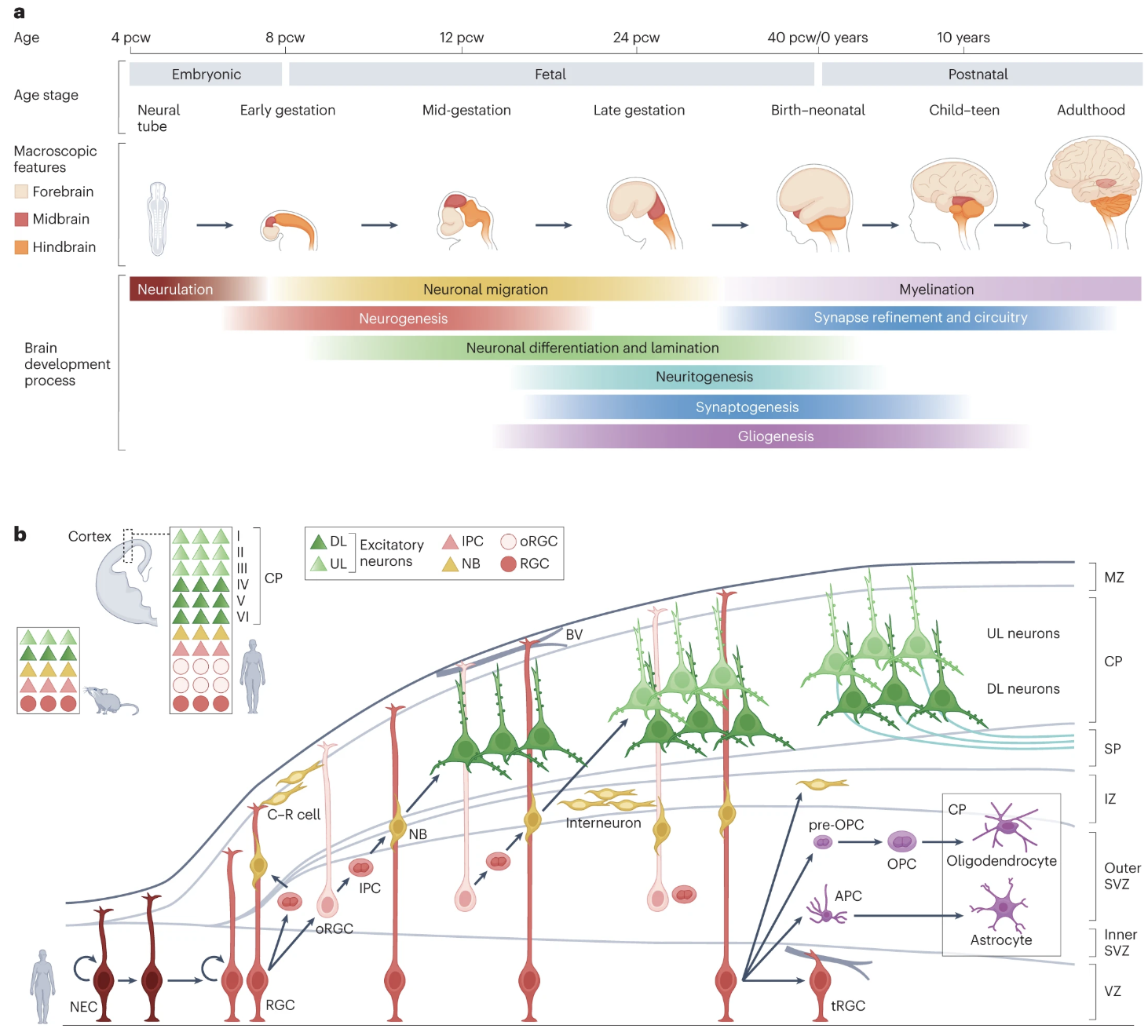
- How the brain develops (i.e. the longitudinal sequence of events between birth and maturation), shown in Figure 2.1.
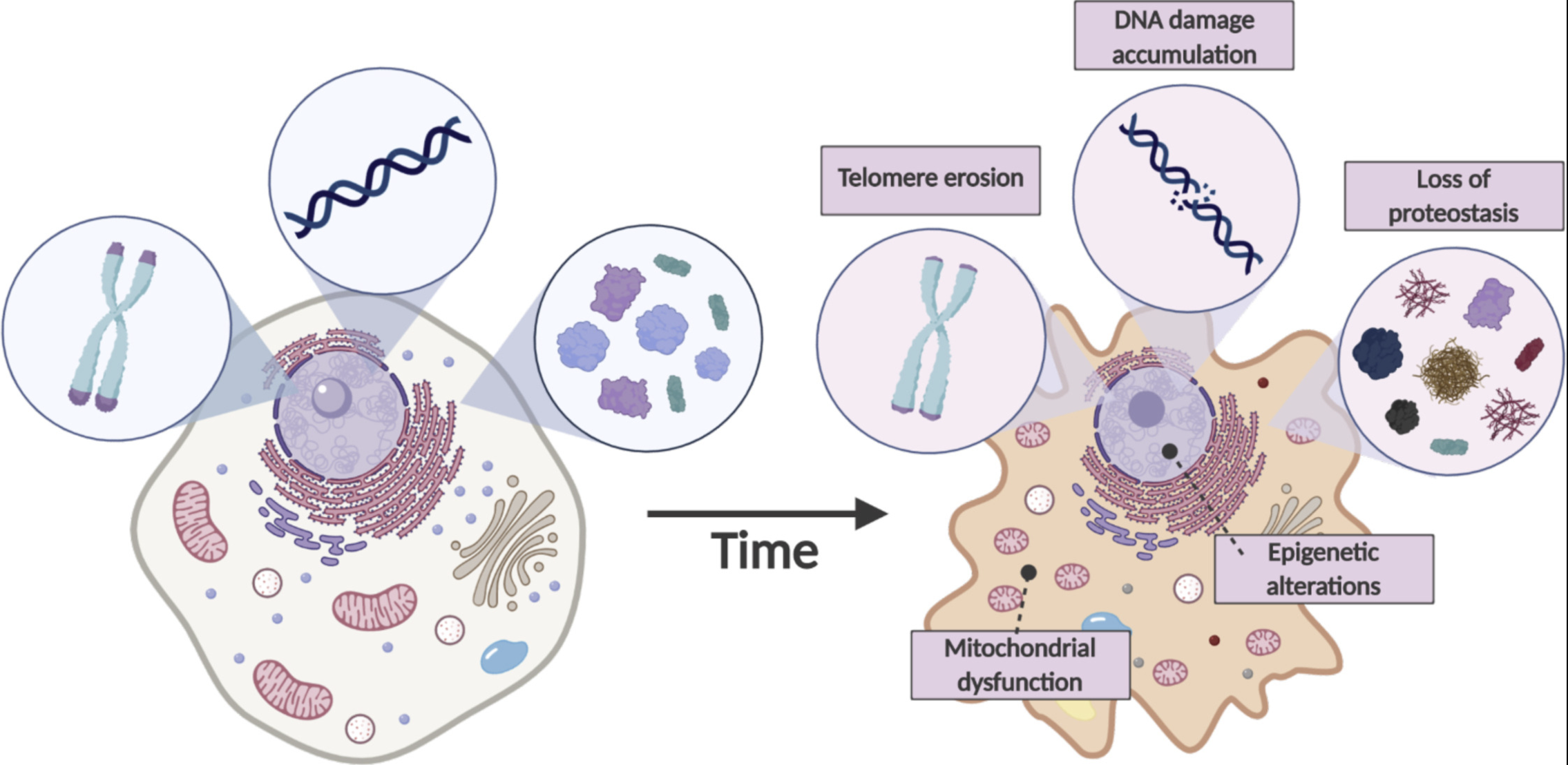
- How microglia in the brain gain or lose certain functions during ageing, shown in Figure 2.2.
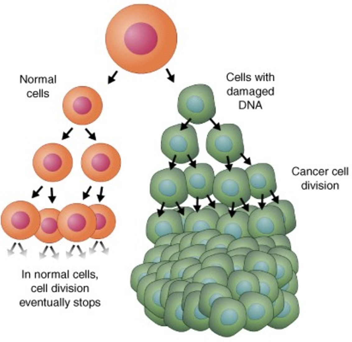
- Why certain cells (i.e. cancer cells) divide uncontrollably, see Figure 2.3.
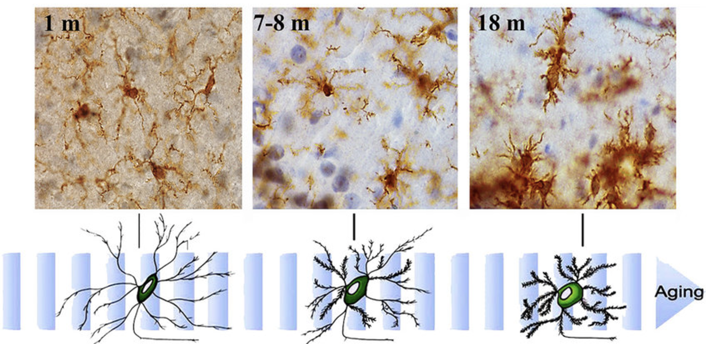
What are the functional consequences of this? (Von Bernhardi, Eugenı́n-von Bernhardi, and Eugenı́n 2015)
2.1.3 How “omics” comes into the picture
To answer cell-biology questions we leverage different omics to learn clues about
1. the cellular functions of a biological system, and
2. how those functions change during disease, ageing, etc.
All these omics are related:
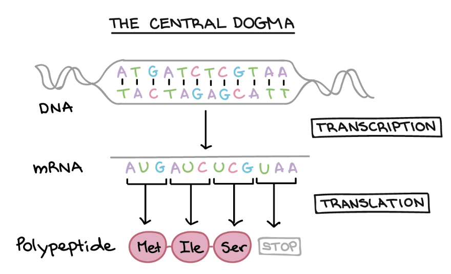
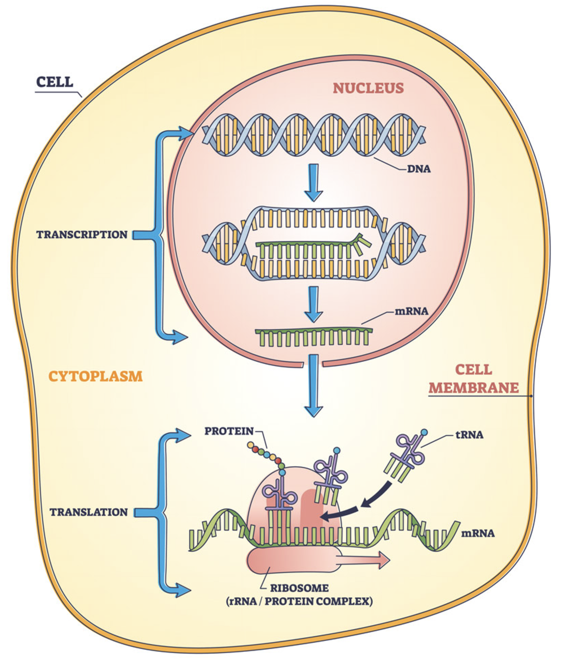
- The central dogma of biology (DNA → RNA → protein) is illustrated in Figure 2.4 and Figure 2.5, linking the three most fundamental omics.
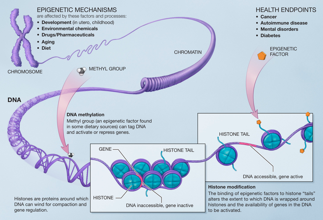
- The epigenome, shown in Figure 2.6, comprises chemical modifications to DNA and histone proteins that regulate gene expression yet are not part of the DNA itself. The figure highlights three commonly studied features: DNA accessibility, DNA methylation, and histone modifications.
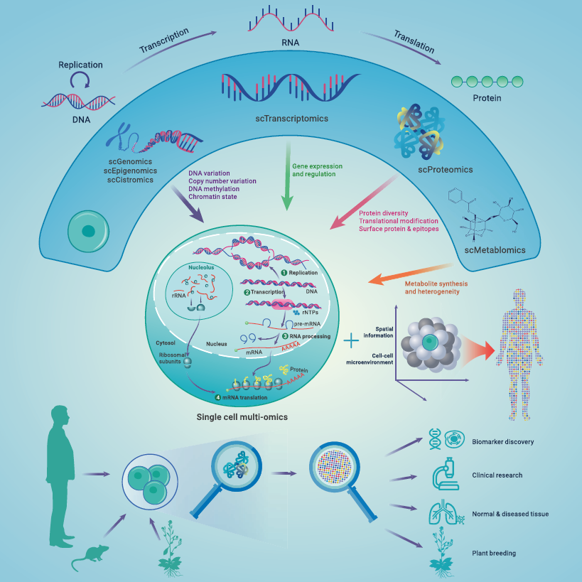
These layers are summarised in Figure 2.7.
Remark (Personal opinion: Biology is constantly revising the details).
Statistical knowledge is rarely revised – its instead mostly refined. We know properties that generalize to much broader settings (i.e., less statistical assumptions) and much more refined statistical rates for the settings studied two decades ago. (1) There’s little revisions, since once someone proves a statistical theorem, it is very unlikely for it to get disproven in the future. (2) Statistics generally focuses on what happens in an “average/typical” scenario.
Biology, in comparison, has many revisions and refinements. There’s a couple reasons for this: (1) Biology research is driven by technology. Hence, as we can image/sequence/profile new aspects of a cell, design new model organisms, or collect more data, we might revise a lot of understanding of how cells work. (2) While there are broad biological mechanisms that generally hold true, many diseases occur when the general biological principle no longer holds true. For this reasons, a lot of cell biology research is about these exceptions, which cause us to question how universally true a biological mechanism is. (As a simple example – we’re taught humans have 46 chromosomes. However, many conditions such as Down Syndrome, originate from having an abnormal number of chromosomes.)
Remark (All the omics we will study in this course are matrices).
One of major missions of this course is to answer the following question: Every omic is represented as a matrix (generally, where the rows are cells, and columns are certain features, depending on the omic). In that case, how come some statistical methods designed for one omic isn’t applicable for another omic?
While there are certain statistical answers to this question, most of the answers are based on biology. Certain methods rely on a specific biological premise, and that premise becomes hard to justify as you switch from one omic to another.
This is not too dissimilar from a causal analysis. In a causal analysis, the reason certain features get labeled as a confounder, treatment, outcome, instrumental variable, mediator, etc. relies on the context.
2.2 What do we hope to learn from single-cell data?
2.2.1 Basic biology
Single-cell data offer a transformative lens to study the fundamental processes of life at unparalleled resolution. Unlike bulk data, which averages signals across populations of cells, single-cell technologies allow researchers to examine the diversity and complexity of individual cells within a tissue or organism. This level of detail provides insights into key biological phenomena, such as cellular differentiation during development, the plasticity of cell states in response to environmental cues, and the organization of complex tissues. For instance, single-cell RNA-sequencing (scRNA-seq) has uncovered new cell types in the brain and immune system, challenging traditional classifications and offering a more nuanced understanding of cellular identities and functions. These insights are essential for constructing more accurate models of how life operates at a cellular level.
Many of the examples shown in Figs. Figure 2.1–Figure 2.2 are basic biology questions. Two additional examples are shown in Figure 2.8 and Figure 2.9.
2.2.2 Benchside-to-bedside applications
Single-cell data have enormous potential to revolutionize clinical practice by bridging molecular biology and medicine. After learning basic biology, the next stage is to use our newfound understanding to advance treatments. (We typically call this translation research, to denote translating our basic biology knowledge to therapeutic improvements.) This is also called benchside (for the wet-bench, i.e. laboratory setting) to bedside (for the hospital setting).
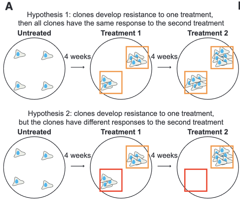
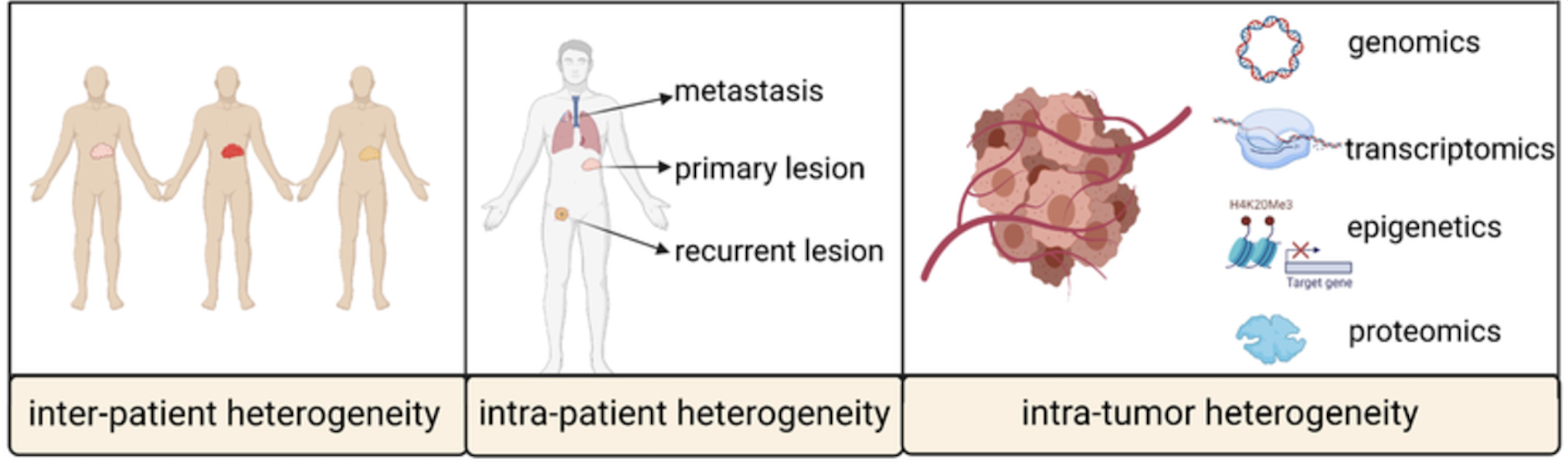
By mapping cellular heterogeneity in diseased and healthy tissues, researchers can identify specific cell populations driving disease progression and therapeutic resistance. For example, in cancer, single-cell analyses have uncovered rare tumor subclones that evade treatment, providing critical targets for drug development. Similarly, in autoimmune diseases like rheumatoid arthritis, single-cell profiling of synovial tissues has identified inflammatory cell states that correlate with disease severity and treatment response. Beyond diagnostics, this technology enables precision medicine by tailoring treatments to the molecular profiles of individual patients. As single-cell approaches continue to evolve, they are poised to refine drug-discovery pipelines, improve vaccine design, and ultimately transform how diseases are diagnosed and treated.
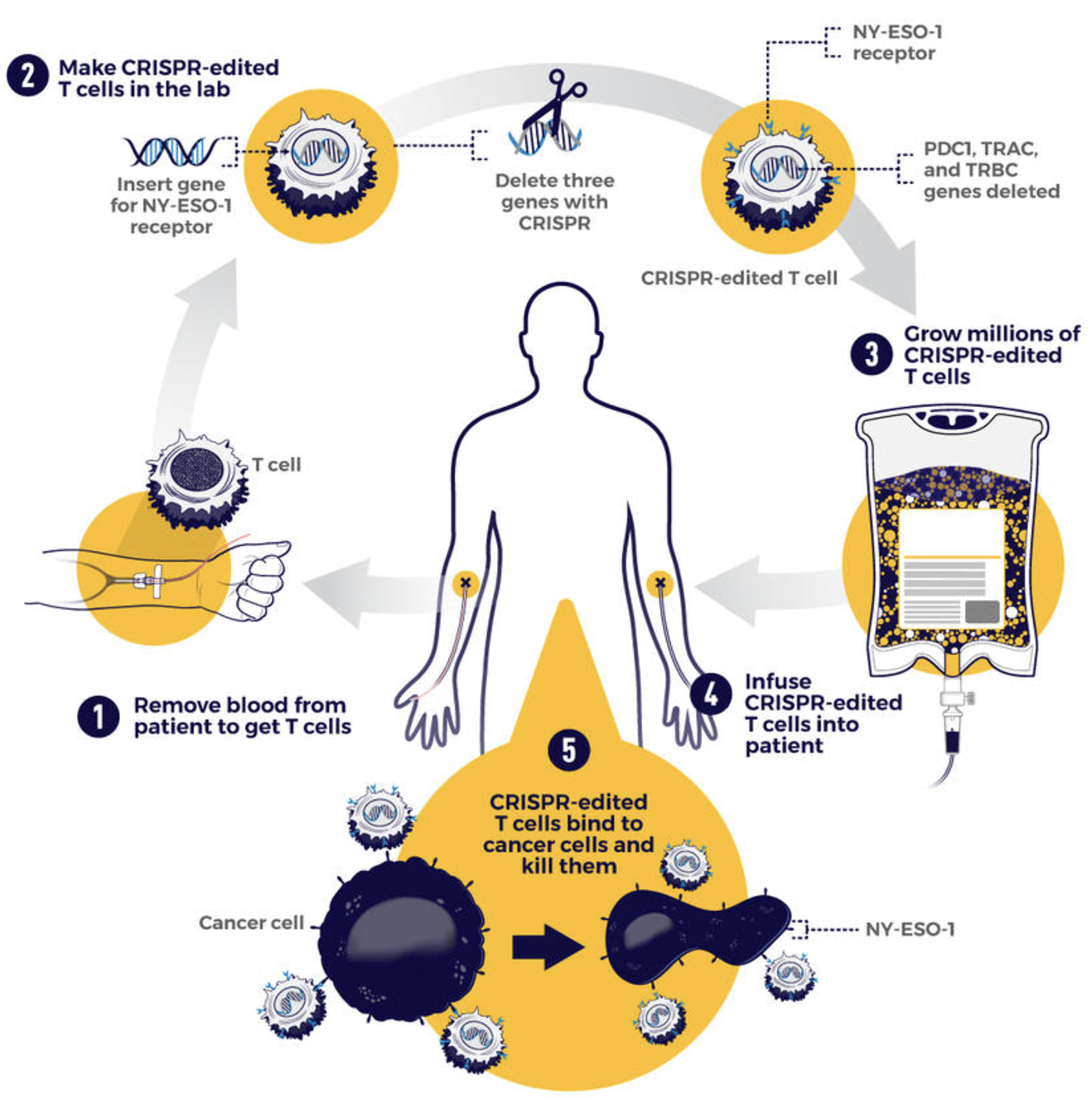
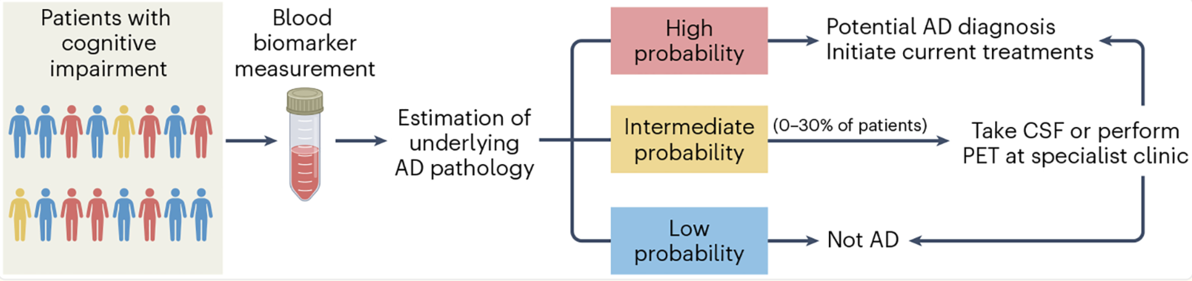
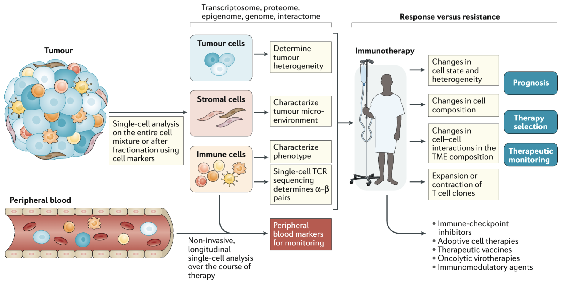
There are a few ways this typically happens. Figure 2.10 shows one example, where single-cell research helps identify the specific cell types and specific edits needed to improve cellular function. Figure 2.11 shows another example, where understanding the cellular functions, we can improve how conventional methods can be used to measure more accurate biomarkers. Cancer research has been (by far) the biggest beneficiary of single-cell research, and Figure 2.12 illustrates how single-cell improves cancer therapies.
2.2.3 What existed prior to single-cell data?
Western blots and flow cytometry.
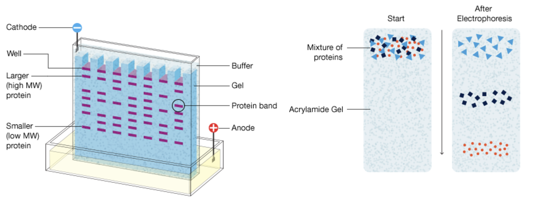
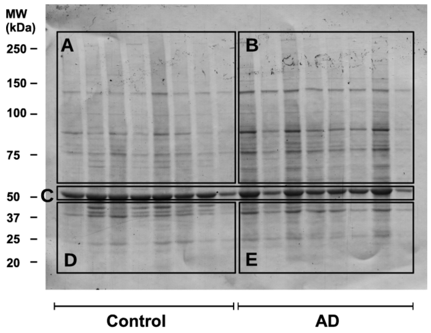
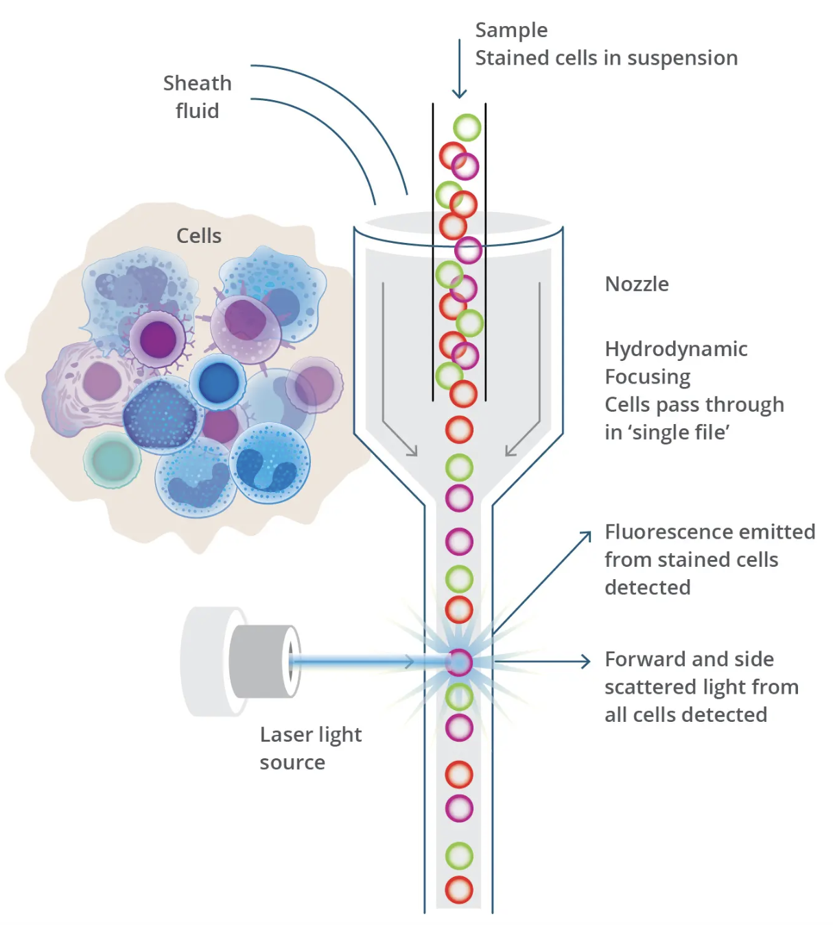
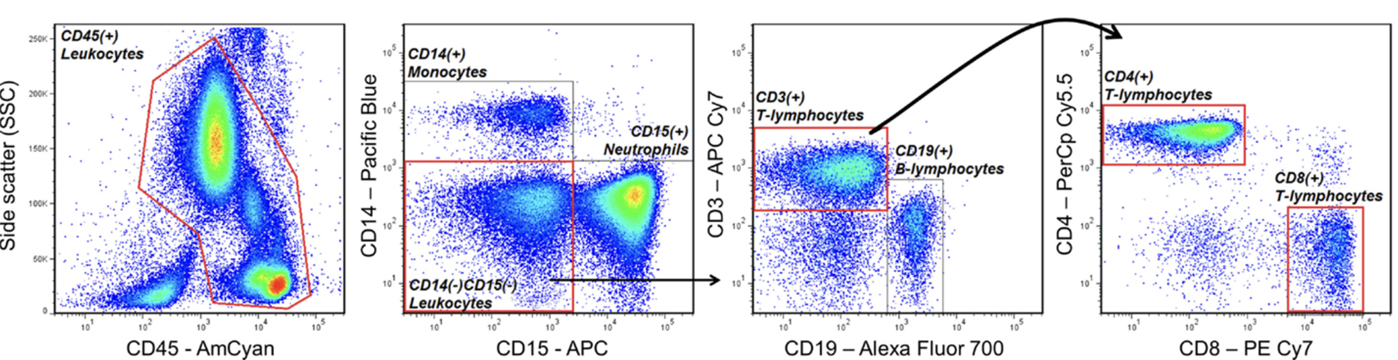
Before the advent of single-cell technologies, biological research relied heavily on methods like western blots and flow cytometry to study cells and molecules. Western blotting (shown in Figure 2.13 and Figure 2.14), developed in the late 1970 s, enabled researchers to detect and quantify specific proteins in a sample, providing insights into cellular pathways and protein-expression levels. However, this technique required lysing entire tissues or cell populations, averaging the signals from thousands or millions of cells. Flow cytometry (shown in Figure 2.15 and Figure 2.16), emerging in the 1980s, represented a major step forward by allowing researchers to analyse individual cells’ physical and chemical characteristics in suspension. While flow cytometry offered single-cell resolution, it was limited to analysing predefined markers and could not capture the full complexity of cellular states or gene expression.
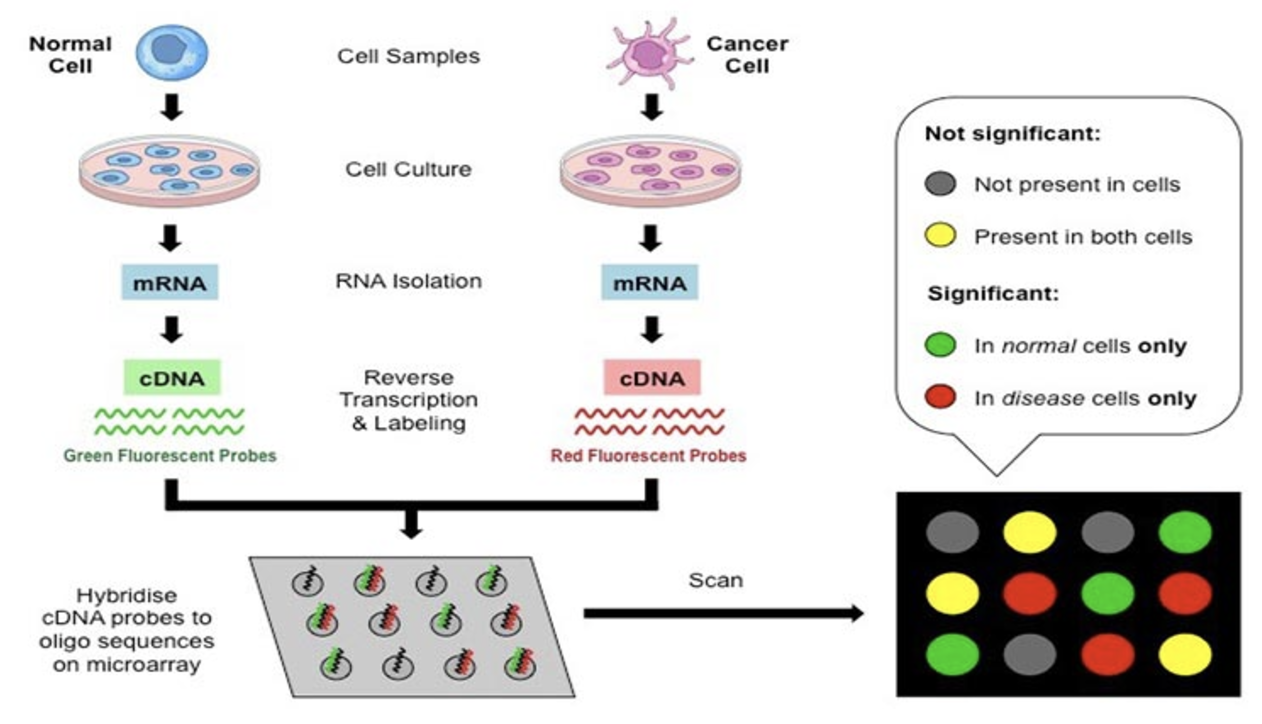
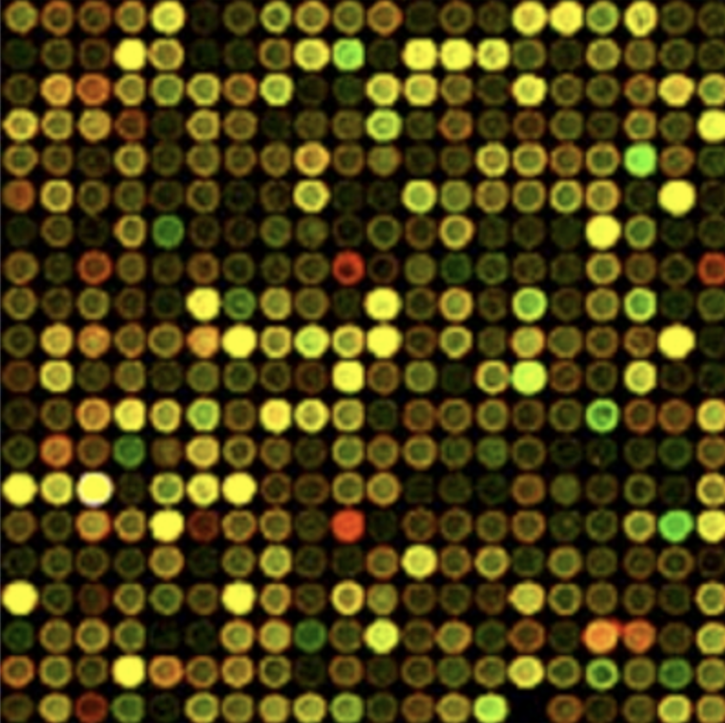
Microarray technology.
The 1990s marked the rise of microarray technology (shown in Figure 2.17 and Figure 2.18), which allowed scientists to measure the expression levels of thousands of genes simultaneously. Microarrays revolutionised transcriptomics by enabling high-throughput studies of gene activity in various conditions, tissues, and diseases. Despite its transformative impact, microarray analysis was fundamentally a bulk method, averaging signals across all cells in a sample. It is also based on light intensity, which can be tricky to extract consistently. These limitations obscured cellular heterogeneity, especially in complex tissues where distinct cell types or states contribute uniquely to biological processes or disease mechanisms.
Remark (Personal opinion: the close history between microarrays and high-dimensional statistics).
Historically, the rise of microarray data spurred advances in high-dimensional statistics — e.g. the Lasso (Tibshirani et al. 2005), gene-expression classification for leukaemia (Golub et al. 1999), and empirical-Bayes multiple testing (Efron and Tibshirani 2002).
Bulk sequencing technologies.
In the 2000s, bulk sequencing technologies for DNA and RNA emerged, further advancing the study of genomes and transcriptomes. RNA-sequencing (RNA-seq) became a powerful tool for capturing the entire transcriptome with greater accuracy and dynamic range than microarrays. Similarly, DNA sequencing enabled comprehensive studies of genetic variation, from point mutations to structural alterations. However, like microarrays, bulk sequencing aggregated signals across many cells, masking rare cell populations and the heterogeneity critical to understanding dynamic processes such as tumour evolution or immune responses. These bulk techniques laid the groundwork for single-cell methods by driving innovations in high-throughput sequencing and data analysis, which would later be adapted for single-cell resolution.
2.3 When did single-cell data become popular, and how has the technology advanced?
2.3.1 The rise of single-cell data
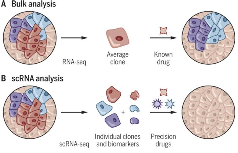
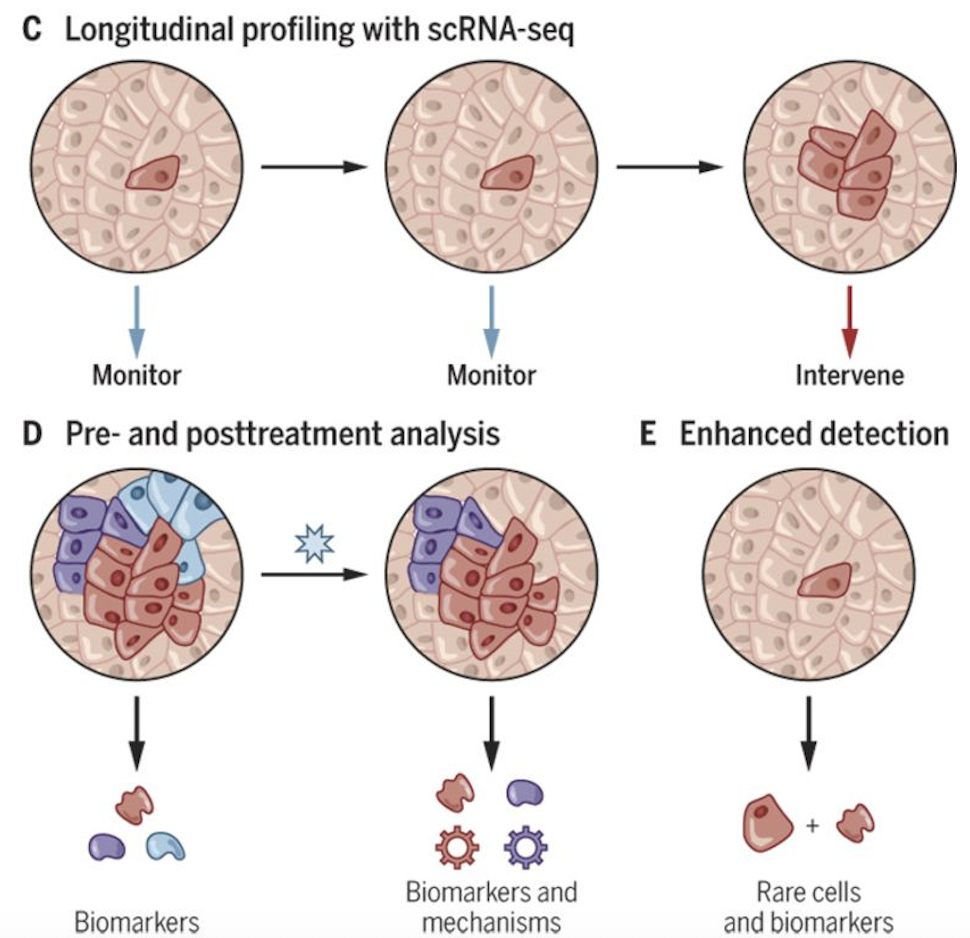
Single-cell data began gaining prominence in the early 2010s, fuelled by advances in microfluidics and next-generation sequencing. Single-cell RNA-sequencing (scRNA-seq), pioneered around 2009 – 2011, was among the first methods to achieve widespread adoption. It enabled measurement of gene expression in individual cells, uncovering heterogeneity that bulk analyses masked. Early applications revealed new cell types and states, reshaped our understanding of development, and identified rare populations in cancers and neurodegenerative disorders. Popularity grew as throughput increased, costs fell, and workflows became standardised.
Figure 2.19 and Figure 2.20 contrasts bulk and single-cell sequencing. Figure 2.21 shows how single-cell data tease apart different sources of heterogeneity.
2.3.2 Expansion into other omics and spatial technologies
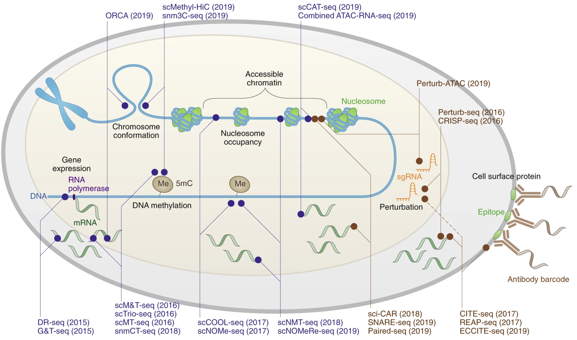
Building on single-cell transcriptomics, the field rapidly expanded into other omics. Single-cell proteomics allows detailed analysis of protein expression and signalling pathways. Single-cell ATAC-seq profiles chromatin accessibility; Hi-C and related methods reveal 3D genome architecture. Spatial transcriptomics connects gene expression with tissue context. CRISPR-based single-cell screens enable high-throughput perturbations, and lineage-tracing barcodes add a temporal dimension, charting cell ancestry in development and disease. Together, these advances transformed single-cell biology into a multi-dimensional, integrative discipline.
Many of these technologies appear in Figure 2.22.
2.4 What is the role of a biostatistician in a wet-lab / clinical world?
Cell biology is vast – especially for students trained primarily in statistics or biostatistics. Many disciplines intersect with cell biology. For example:
- Statistics / Biostatistics – statistical models for complex biological processes; translation between maths and biology
- Computational biology – scalable computation, leveraging public data
- Bioinformatics / Genetics – tools that draw on large‐consortium resources
- Epidemiology – population-level data and policy recommendations
- Bioengineering – new laboratory technologies for cheaper/faster measurement or imaging
- Biology – mechanistic studies in model organisms
- Biochemistry / Molecular biology – structure, function, interactions of specific molecules
- Wet-bench medicine – disease mechanisms via tissues, models, cell lines
- Clinical-facing medicine – patient treatment and real-world sample collection
- Pharmacology – integrating evidence to design new drugs and therapies
Given so many players, what does a biostatistician contribute?
2.4.1 How a biostatistician perceives the world
Give me a concrete (ideally cleaned) dataset: the larger the better—and I will analyse it from many angles.
Causality: A mathematically stricter notion than correlation, usually via (1) counterfactual reasoning, or (2) a directed-acyclic-graph picture of how variables relate.
Remark (Personal opinion: statistical causality for cell biology is extremely difficult). Obstacles: (i) tracking the same cell over time is impossible because sequencing lyses it; (ii) longitudinal human tissue samples are rare. Strong modelling assumptions can help but must withstand biological scrutiny. The bottleneck is often data, not maths—ambitious statisticians who learn enough biology still have a fighting chance.
Remark (Single-cell methods are largely an “associative” world): Most single-cell analyses discover mechanisms that are statistically correlational; the causal proof comes from experiments and biology.
The research inquiry starts and ends with a method: (How to integrate modalities? learn a gene-regulatory network? perform valid post-clustering tests?) Start with a statistical model and a parameter of interest \(\theta^*\), then typically:
Develop a novel estimator of \(\theta^*\), explaining why current methods fail (e.g. lack robustness, accuracy, power, or are heuristic). Focus on statistical logic: A clear, simple mathematical intuition should show the gap and how the new method fills it.
Prove theorems showing the estimate \(\hat\theta\) converges to \(\theta^*\) under stated assumptions. Focus on consistency & convergence: More data should provably yield more accurate results (often the highlight of a statistics paper).
Simulations demonstrating that when the true \(\theta^*\) is known, \(\hat\theta\) beats competing estimators across many settings. Illustration via benchmarking: Empirically recover the correct answer more often than existing methods.
Real-data demonstration showing results align with known biology or provide biologically sensible new insights. Focus on practicality: The method must work in real scenarios mirroring its target audience.
Mindset: deliver a reliable tool that others can trust as-is. Human validations are often impractical; guard-rails and diagnostics are vital.
Why biostatisticians need wet-lab biologists / clinicians: We rarely generate data ourselves, so collaborators supply (i) exciting data with novel questions, (ii) biological context for sensible assumptions, and (iii) experimental validation of statistical findings.
2.4.2 How a wet-lab biologist / clinician perceives the world
Experiments, experiments, experiments: Carefully controlled—even if small—to make downstream analysis straightforward.
Causality comes from a chain of experiments. Suppose we study a gene’s role in disease:
Temporal evidence, such as change in gene expression preceding a change in cell phenotype. A causal mechanism should occur before the phenotype.
Biological logic providing explanation of the underlying mechanism (binding factors, protein function, evolutionary rationale, etc.). For example, there must be a coherent pathway from gene → protein → phenotype.
Universality of how the described association persists across cell lines or organisms. A causal mechanism should be discoverable in other systems (extent depends on how general the logic is). This is offten the highlight of a biology paper.
Validation, such as knocking out the gene alters the outcome, whereas similar genes do not. For example, perturbing the specific gene (not its close counterparts) changes the outcome.
Inquiry starts and ends with a biological hypothesis: Large intellectual effort goes into proposing explanations and designing experiments to rule them in or out.
Mindset: Assemble overwhelming evidence for a mechanism, combining careful experiments and biological logic.
Why wet-lab scientists need biostatisticians: Data are now complex and plentiful; exhaustive experiments for every hypothesis are infeasible. Statistical methods can (i) account for data & biological complexity and (ii) prioritise hypotheses worth experimental investment.
So how does a biostatistician develop computational / statistical methods for cell biology?
- Biological context – What is the biological system and the “north-star” question? Which premises are accepted, which ones are to be tested, and why is it important to understand this mechanism better?
- Technology, experiment, data – How are data collected and why did you choose this particular {technology, experiment, data} trio? What technical artefacts arise?
- Boundaries of current tools – Simple analyses first: what “breaks” in existing workflows? Is there preliminary evidence a new computational method would do better?
- Statistical model – What is the insight that a different computational method could interrogate the biology better? (Here the statistics training begins.)
- Develop a method & show robustness – Robustness can be defined numerically (i.e., noise tolerance) or biologically (i.e., applicable across contexts/environments). Often, the biological question you study lacks a ground truth, so validity arguments lean on biological logic.
- Uncover new / refined biology – Does the method advance our biological understanding? How confident are we that findings generalise beyond the original {technology, experiment, data} trio? (This is usually the crown-jewel of your computational biology paper – it’s not necessary your specific analyses, but the potential that your tool can be used on other biological studies beyond what you’ve demonstrated your method on.)