5 ‘Single-cell’ proteomics
Foray into deep learning and multi-omic integration
5.1 Review of the central dogma
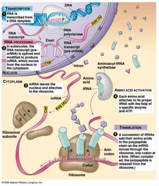
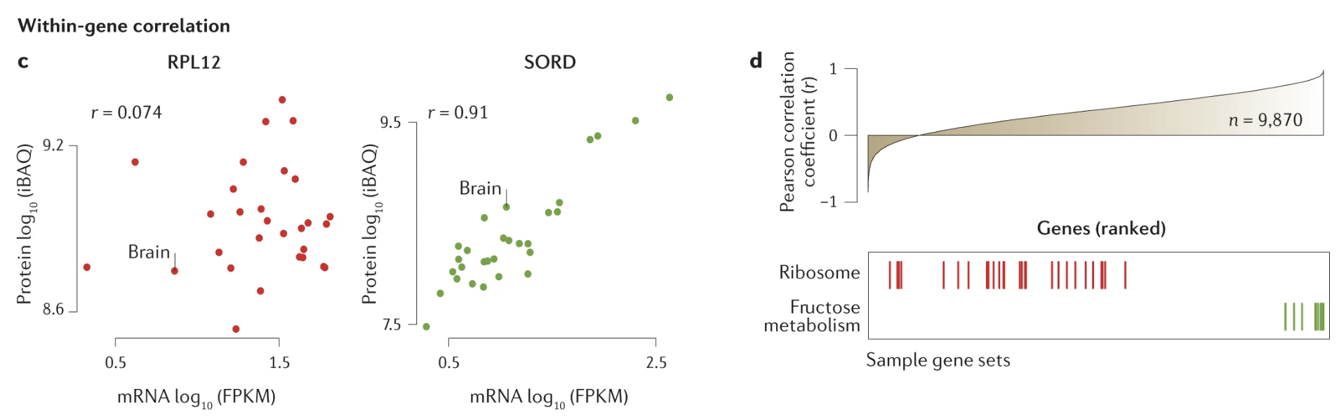
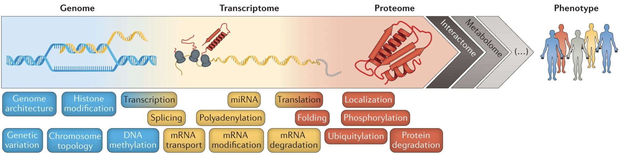
The central dogma of molecular biology outlines the flow of genetic information within a cell: DNA is transcribed into RNA, and RNA is then translated into protein (see Figure 5.1). Specifically, coding genes in DNA are transcribed into messenger RNA (mRNA), which serves as a template for protein synthesis. During translation, mRNA sequences are read in sets of three nucleotides, known as codons, each corresponding to a specific amino acid. These amino acids are then linked together to form proteins, which carry out a vast array of functions within the cell. While this process provides a foundational framework, it is a dramatic over-simplification. As we’ll explore later in the course, the correlation between a gene and its corresponding protein levels is often surprisingly low, highlighting the complexity of gene expression regulation.
Understanding proteins is crucial because they are the primary effectors of cellular function. Most cellular activities — whether structural, enzymatic, or signaling—are mediated by proteins. While RNA intermediates, such as mRNA, play important roles in carrying genetic information, the majority of RNA fragments never leave the cell, with a few exceptions like extracellular RNA in communication. Proteins, however, directly influence both intracellular processes and extracellular interactions. Given the weak correlation between genes and proteins and the central role proteins play in biological function, studying proteins arguably provides a more direct and meaningful insight into cellular and organismal behavior. This dual perspective on the central dogma will frame much of our exploration in this course.1
5.2 Other ways to study proteins that we’re not going to discuss here
5.2.1 So You Heard About AlphaFold…
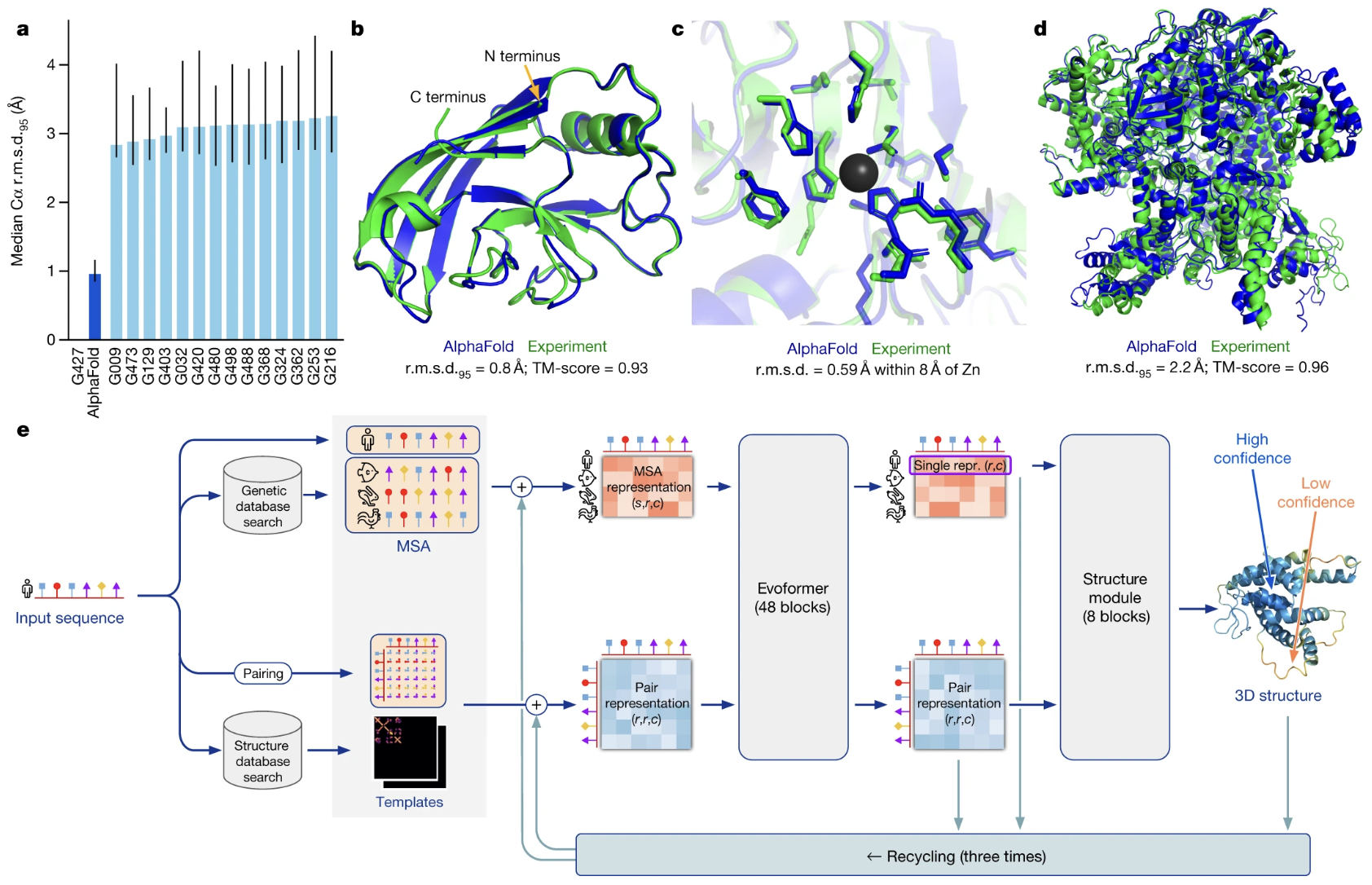
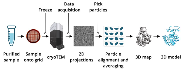
AlphaFold (see Figure 5.4) represents a revolutionary advancement in computational biology, designed to predict the three-dimensional structure of proteins from their amino acid sequences2. Historically, determining protein shapes required experimental techniques like X-ray crystallography, cryo-electron microscopy (EM) (see Figure 5.5), or nuclear magnetic resonance (NMR), which are resource-intensive and time-consuming. AlphaFold uses deep learning and structural biology insights to achieve high accuracy.
However, significant challenges remain. There are still many open questions on how specific genetic modifications impact protein folding, how proteins dynamically change their conformation, or how they interact with other molecules such as DNA or other proteins. Additionally, ongoing developments in using large language models are showing promise in predicting not only shape but also potential functions directly from amino acid sequences.
5.2.2 Other Methods: Flow Cytometry, Spatial Proteomics, and FISH
While AlphaFold focuses on protein structure, methods like flow cytometry and spatial proteomics explore proteins in their functional and cellular contexts. Flow cytometry, sometimes considered the “original” single-cell data method, measures the expression of surface and intracellular proteins across thousands of cells, providing rich insights into cellular heterogeneity. Spatial proteomics and techniques like fluorescence in situ hybridization (FISH) take this further by localizing proteins and RNA within tissue contexts, enabling researchers to map molecular interactions in their native environments. These approaches highlight the versatility of protein studies, from understanding their structure to dissecting their function and distribution in complex systems. While not the focus of this course, these methods are invaluable in expanding our understanding of proteins and their roles in biology.
5.3 Just a very brief blurb about the passive and adaptive immune response
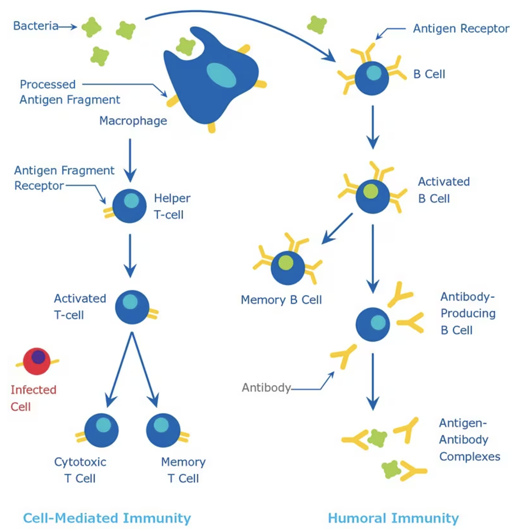
The immune system functions as a highly coordinated defense network, designed to detect foreign invaders such as pathogens and viruses, mount an appropriate response, and retain a memory of the invader for faster recognition in the future. This response involves two primary arms: the innate (passive) immune response, which provides a rapid but non-specific reaction, and the adaptive immune response, which is slower but highly specific and long-lasting (Figure 5.6). The innate immune system acts as the first line of defense, utilizing macrophages and dendritic cells to patrol tissues, engulf pathogens, and present antigens to activate the adaptive response. These antigen-presenting cells serve as surveillance officers, alerting the adaptive immune system to potential threats.
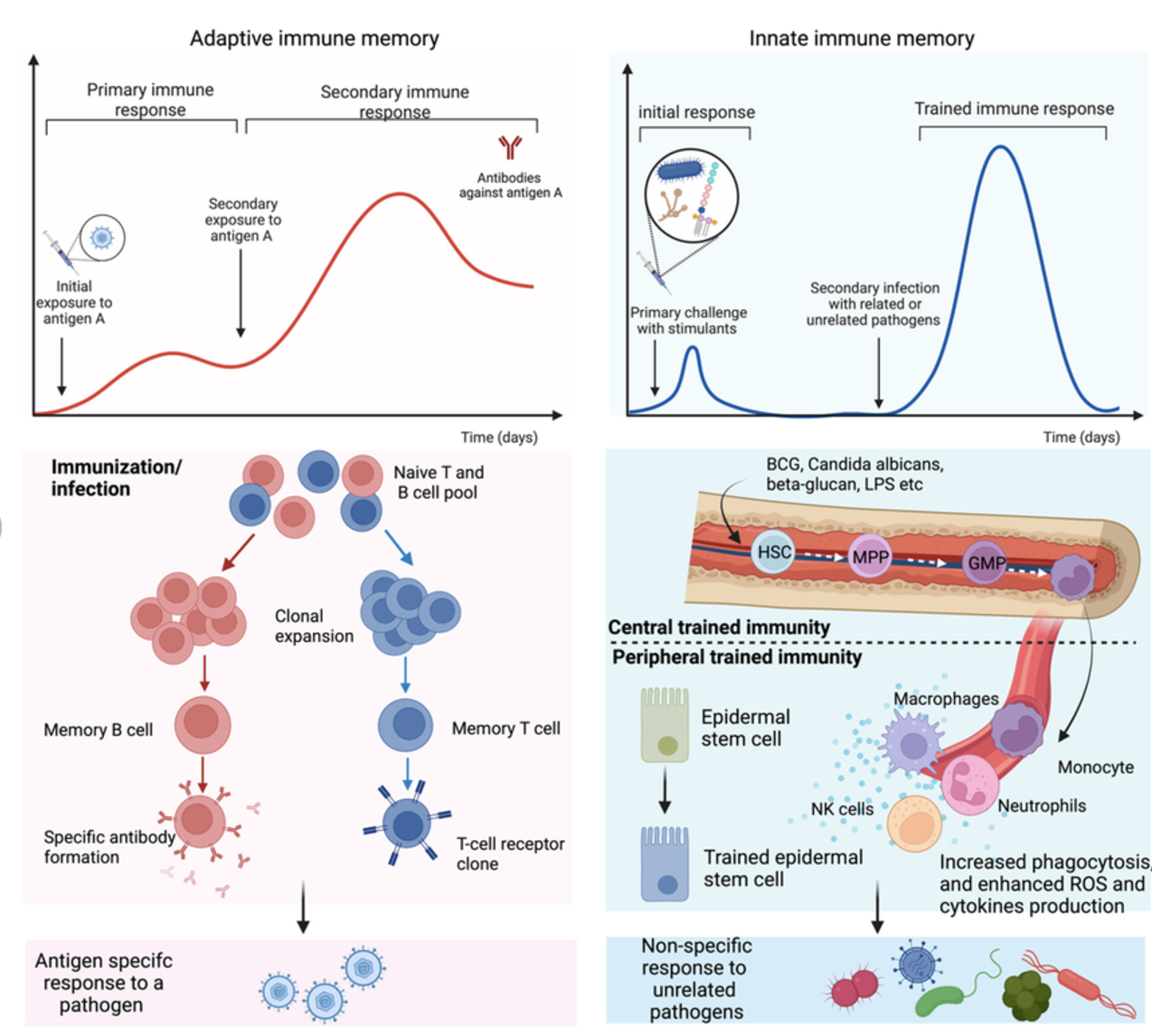
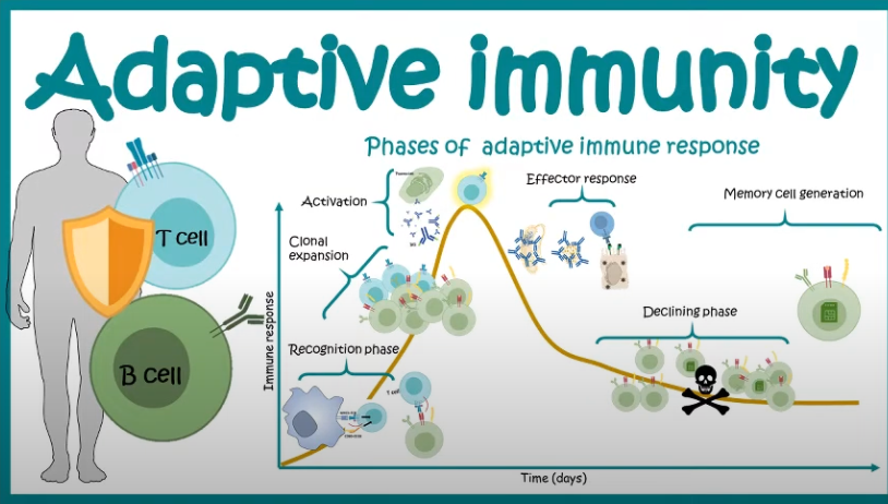
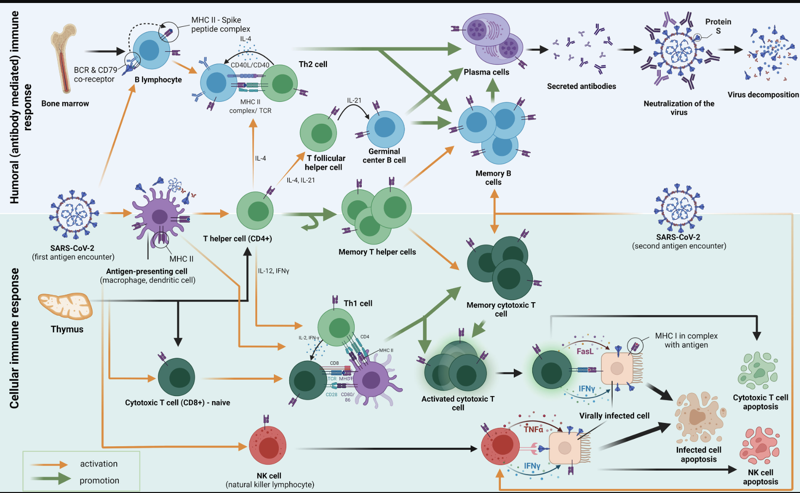
Once the adaptive immune system is activated, a complex cellular expansion process takes place. T-cells and B-cells, the key players of adaptive immunity, undergo rapid division to generate an army of pathogen-specific defenders (Figure 5.7; Figure 5.8). B-cells produce antibodies that neutralize the invader, while T-cells can either directly kill infected cells or help orchestrate the immune response. Once the threat is eliminated, the expanded immune cell population undergoes programmed cell death to prevent excessive immune activity, leaving behind a small number of memory cells that provide long-term immunity. This cycle of surveillance, expansion, and contraction resembles a law enforcement system that transitions from routine surveillance (innate immunity) to full military mobilization (adaptive immunity) when an invasion occurs, ensuring both immediate and long-term protection.
5.4 CITE-seq: Sequencing mRNA alongside cell surface markers, simulteaneously
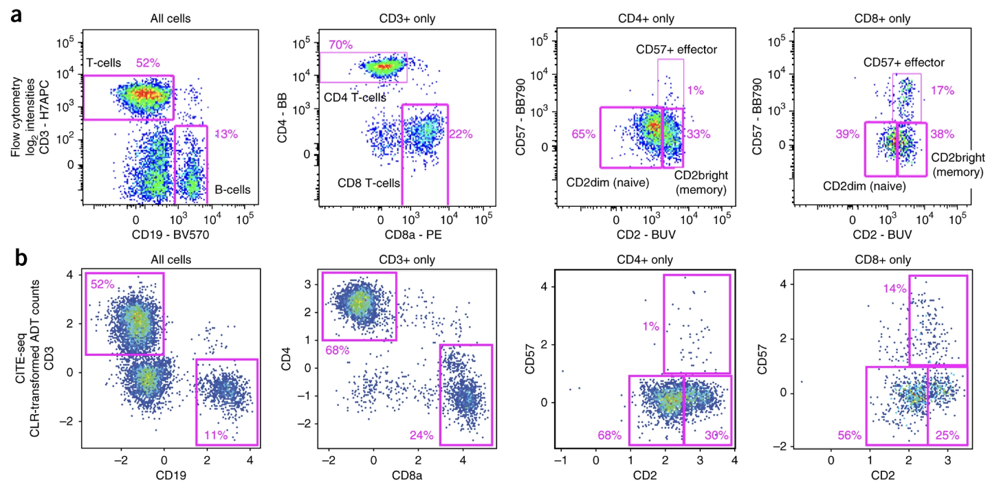
CITE-seq (Cellular Indexing of Transcriptomes and Epitopes by sequencing) (stoeckius2017simultaneous?) extends the capabilities of single-cell RNA-seq by simultaneously measuring messenger RNA (mRNA) and surface protein expression in the same cell. This is achieved by combining traditional single-cell RNA-seq protocols with oligonucleotide-labeled antibodies that bind to specific surface proteins. These oligonucleotides are then sequenced alongside the mRNA, providing a comprehensive view of both transcriptional and protein-level information for each cell.3 See Figure 5.9 for a comparison between the cell populations that are separable with flow cytometry verses the surface proteins in a CITE-seq dataset.
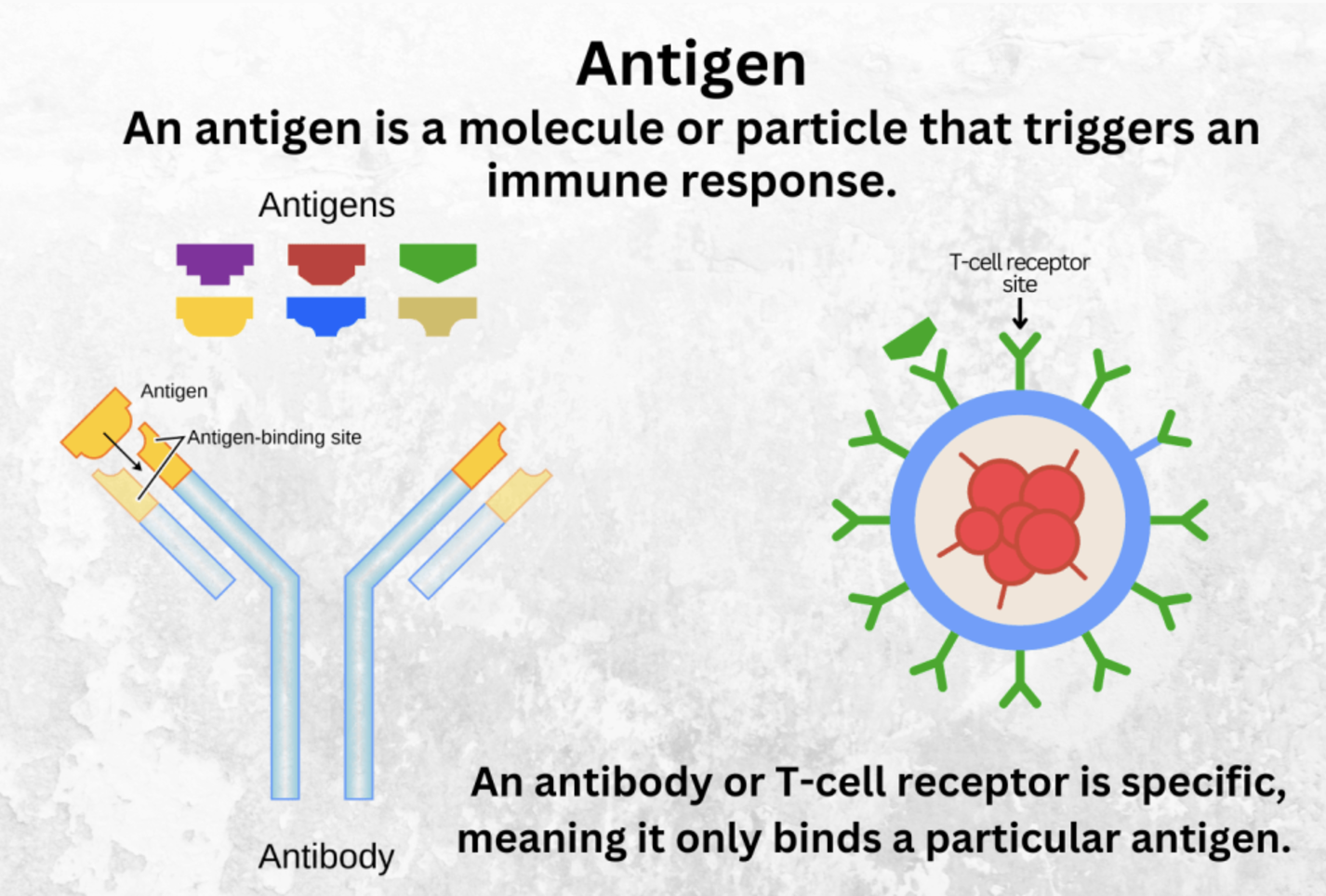
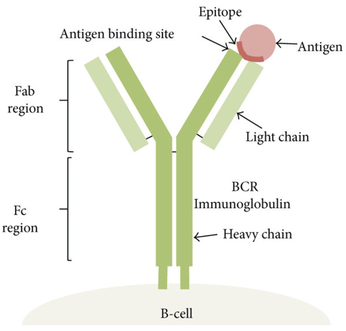
First, some vocabulary: - Antibody and its epitope: An antibody is a Y-shaped protein produced by the immune system that binds specifically to an antigen, which is often a protein or peptide. The part of the antigen that the antibody recognizes and binds to is called the epitope. This interaction is highly specific, allowing antibodies to target unique molecular features of cells, pathogens, or other biological molecules. See (Figure 5.10; Figure 5.11; Figure 5.12).4
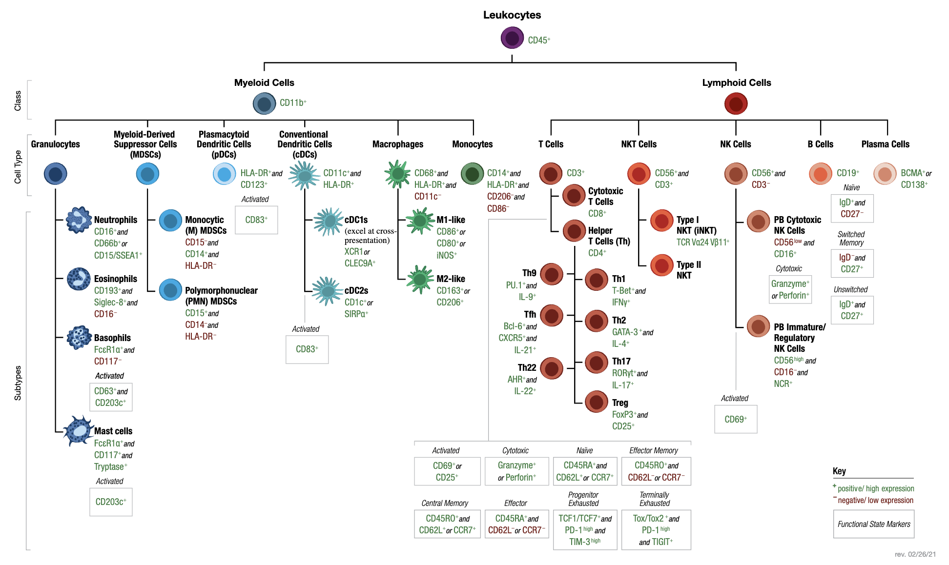
- Surface markers (CDs): Cell surface markers, often referred to as CD (cluster of differentiation) markers, are proteins expressed on the surface of cells that serve as distinguishing features of specific cell types or states. These markers are commonly used in immunology and single-cell analyses to classify and study immune cells. For example, CD4 and CD8 are well-known markers for helper T cells and cytotoxic T cells, respectively. The ability to target CD markers with labeled antibodies is central to techniques like flow cytometry and CITE-seq. See Figure 5.13 for a table of common CDs used to identify immune cells.
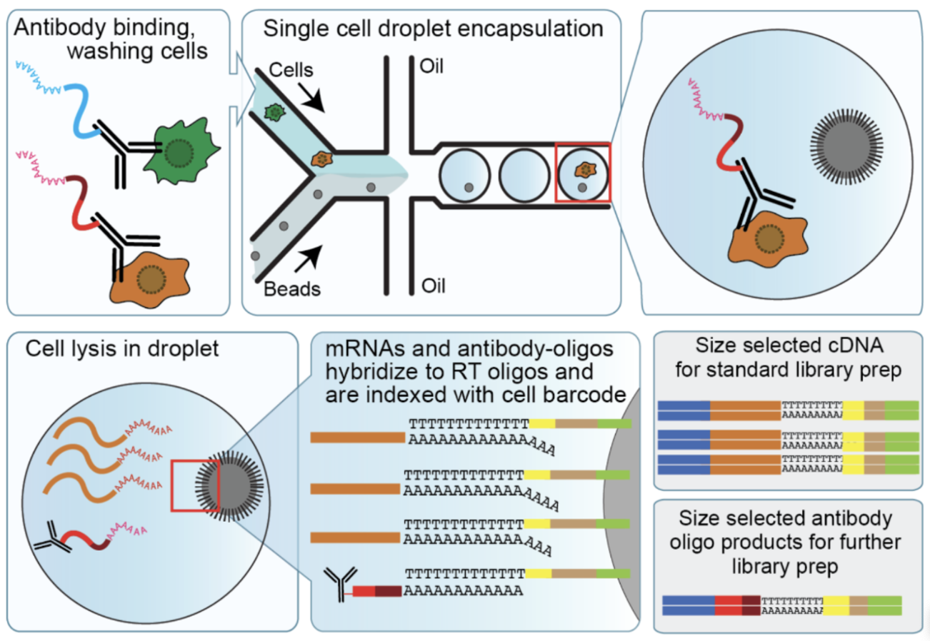
Here is a brief description of the CITE-seq steps (see Figure 5.14):
Tissue dissociation and cell isolation: This step remains identical to traditional single-cell RNA-seq. The tissue of interest is dissociated into a suspension of single cells, and cells are isolated via techniques like fluorescence-activated cell sorting (FACS) or microfluidics. The primary difference comes afterward, when specific oligonucleotide-conjugated antibodies are added to the cell suspension.
Antibody labeling: In this unique step, oligonucleotide-labeled antibodies are used to bind to surface proteins on each cell. Each antibody is tagged with a DNA barcode unique to the specific protein it targets. These DNA barcodes are critical for linking sequencing data back to the corresponding surface proteins.
Droplet formation: Similar to RNA-seq, cells are encapsulated into droplets along with barcoded beads. These beads capture both the mRNA and the antibody-bound oligonucleotides. This simultaneous capture is what makes CITE-seq distinct, as it preserves information about both RNA transcripts and protein markers.
Cell lysis and RNA/antibody capture: Cells are lysed within droplets, releasing both RNA and antibody-conjugated oligonucleotides. The RNA hybridizes to barcoded beads as in traditional RNA-seq. Simultaneously, the antibody-derived oligonucleotides are captured using complementary sequences on the same beads.
Reverse transcription, cDNA synthesis, and amplification: The RNA is reverse-transcribed into complementary DNA (cDNA), while the antibody-derived oligonucleotides are also amplified. This ensures sufficient material for sequencing both modalities.
Library preparation and sequencing: Separate libraries are prepared for the RNA and antibody-derived oligonucleotides, but they are sequenced together on the same high-throughput platform. This co-sequencing ensures that both mRNA and protein data are linked to their respective cells via barcodes.
Mapping, alignment, and data integration: RNA reads are mapped to a reference genome or transcriptome as in traditional single-cell RNA-seq. Antibody-derived oligonucleotide reads, however, are mapped to predefined sequences representing the antibody barcodes. The two data modalities are then integrated, enabling joint analyses of mRNA and protein expression.
Remark 5.1. Why surface markers matter
Surface proteins often provide critical insights into a cell’s phenotype, function, and state that cannot always be inferred from mRNA expression alone. By combining transcriptomics with surface proteomics, CITE-seq enables deeper biological interpretation, such as identifying cell types or states that are transcriptionally similar but phenotypically distinct.
CITE-seq is often performed on immune cells because of their abundance of surface markers, which play a critical role in their biological functions. Immune cells, such as T cells, B cells, natural killer cells, and monocytes, are defined by their expression of distinct surface proteins. These markers are essential for their roles in immune response, cell-cell communication, and recognition of pathogens or damaged cells.
5.4.0.1 A brief note on other technologies
See (gong2025benchmark?) for a comparison between different technologies that measure single-cell transcriptomics and proteomics. See (lischetti2023dynamic?) for some notes about how CITE-seq has been used, or (as examples) its applications in leukemia (granja2019single?) or CAR T therapy (good2022post?).
5.5 A Primer on VAEs
Variational autoencoders (VAE) is a type of deep-learning architecture that is exceptionally common for studying single-cell sequencing data. We’ll build up to this and its application of CITE-seq data slowly, piece-by-piece.
5.5.1 What is an autoencoder?
Input/Output. The input to an autoencoder is the same as any dimension reduction method (like PCA). The input is a matrix \(X \in \mathbb{R}^{n\times p}\) for \(n\) cells and \(p\) features. The output is \(Z \in \mathbb{R}^{n \times k}\), where \(k \ll p\) (where there are \(k\) latent dimensions). We call \(Z\) the embedding. Autoencoders also return the “denoised” matrix \(X' \in \mathbb{R}^{n\times p}\).
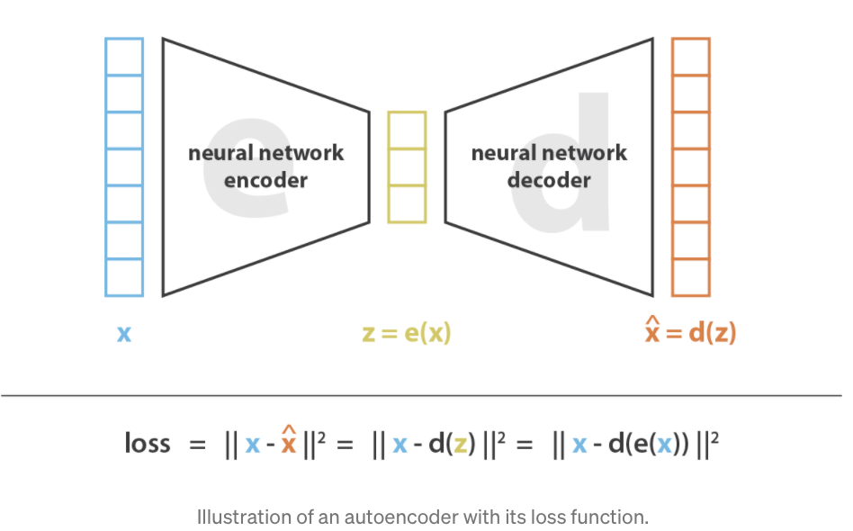
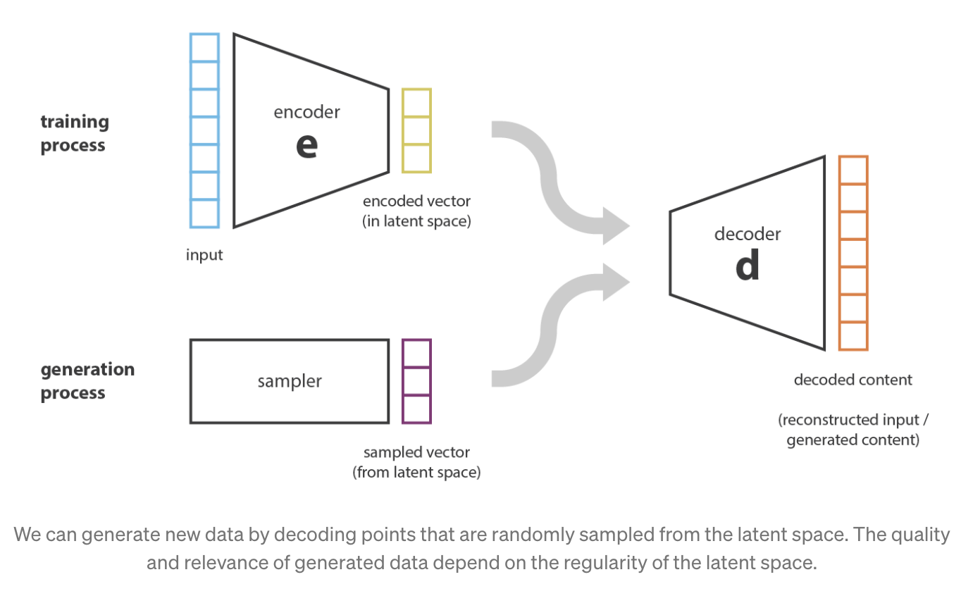
Figure 5.15 and Figure 5.16 illustrate the general structure of an autoencoder. It consists of two key components: an encoder, which maps the input data \(x\) into a latent space representation \(z\), and a decoder, which reconstructs the input \(x\) from the latent variables \(z\).
Some notable aspects: - Linear and non-linear functions: Typically, most of these neural network architectures for AEs are in the following form: for example, let the input for one layer be \(X \in \mathbb{R}^{p}\), and the AE learns a weight matrix \(W \in \mathbb{R}^{p \times K}\). Then the output of that layer (which will become the input for the next layer) is \(\text{ReLU}(XW)\), where ReLU is the Rectified Linear Unit.
Minimizing a “deterministic” loss: As illustrated in Figure 5.15 and Figure 5.16, most AEs typically try to minimize the reconstruction loss (i.e., the difference between the original input and the final output). We’ll see how this changes when we discuss VAEs.
Compression of information: As opposed to most NN architectures, in AEs, the number of units in each layer is smaller than the original dimension (typically called “compression” or “bottleneck”), exemplified in Figure 5.15 and Figure 5.16. In most other NN architectures (e.g., GANs, Convolution NN, Recurrent NN’s), the number of units typically grows. The latent representation for a cell with expression \(X_i \in \mathbb{R}^{p}\) will be called \(Z_i \in \mathbb{R}^{K}\) where \(K \ll p\).
Unsupervised setting: As opposed to most NN architectures, AEs are meant for the unsupervised setting. Unsurprisingly, since most of the statistical theory for NNs is for the supervised setting, our understanding of AEs is much more limited compared to that for other NN architectures.
Relation to PCA: AEs are most similar to PCAs by understanding the reconstruction perspective of PCA Equation 3.5. PCA uses: 1) linear functions to encode and decode the data, and 2) sets the decoder to be exactly the “inverse” of the encoder. In AEs, we can: 1) use non-linear functions (such as ReLU) for more complex transformations of the data, and 2) allow the decoder to be different from the encoder. (The reason why the second point might seem useful will become clear when we explain VAEs below.)
5.5.2 What is a variational autoencoder?
Input/Output. The input and output of a VAE is the same as those of an autoencoder.
Here are some motivating questions:
- Why do we even need to specialize the autoencoder?
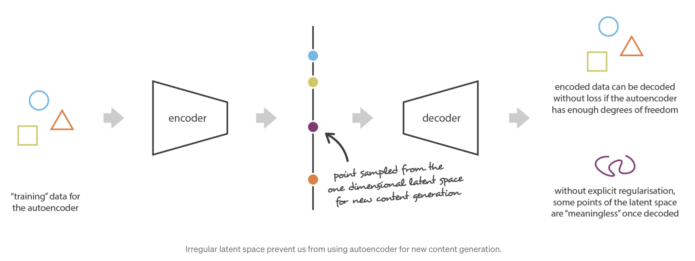
Conceptually, we could hope that an AE can serve as a means to generate new data — simply mix up the learned latent representation \(Z_i\)’s among all the \(n\) cells and use the decoder network to simulate new data. However, due to the highly non-linear nature of NNs, this might result in unexpectedly non-sensible values5. See Figure 5.17 and Figure 5.18.
- How does this impact our conceptual understanding of VAEs?
Hence, this is where we would like to adjust the NN architecture slightly — we want to insert randomness right in the middle of the AE to slightly perturb \(Z\), and we would like the cell’s original expression be similar (“on average”) to its reconstructed expression when its latent representation is slightly perturbed right before it’s decoded. The result is a framework illustrated in Figure 5.19.
Note: The formal way to describe how to set up this framework involves priors, posteriors, etc. We’ll avoid all of this for simplicity, but you can see (kingma2019introduction?) for a formal description.
- What does the architecture for a VAE look like?
A brief quote of what a prototypical VAE is, from (battey2021visualizing?):
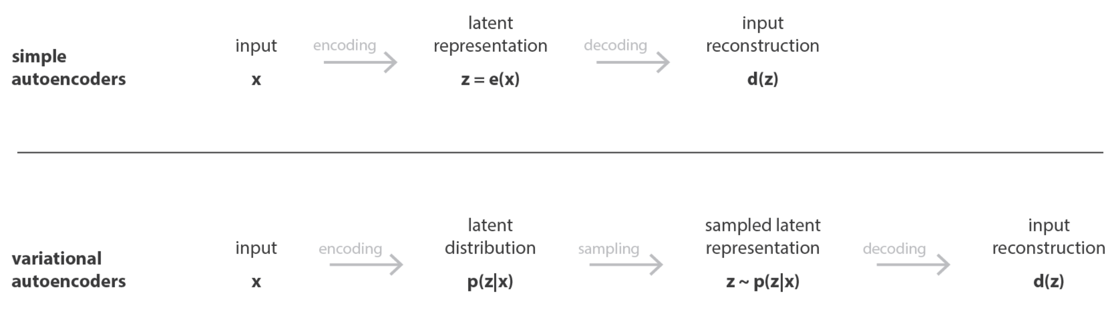
“VAEs consist of a pair of deep neural networks in which the first network (the encoder) encodes input data as a probability distribution in a latent space and the second (the decoder) seeks to recreate the input given a set of latent coordinates (Kingma and Welling, 2013). Thus a VAE has as its target the input data itself.”
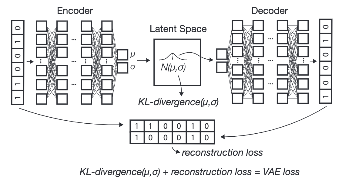
Figure 5.20 and Figure 5.21 illustrate the typical VAE. We see there are now more components — the encoder network “splits” into two types of latent representations, one for the mean of the latent distribution and one for the variance. We then (during the training process) artificially inject Gaussian noise, which “perturbs” our latent representation \(Z\), which is then decoded to get our “denoised” cell’s expression.
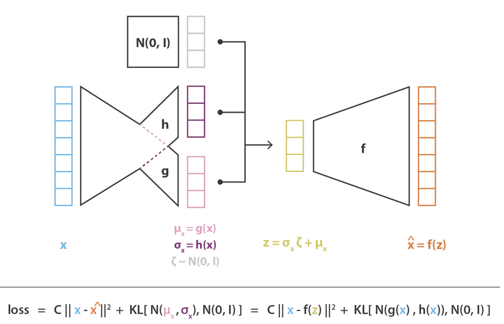
At first, it might seem odd that we’re artificially injecting noise into our training process, as we might think this is harmful to our resulting denoising process6. There are two ways to think about this:
Making the training “more robust”: Despite the decoding network being so highly non-linear, we are trying to ensure that the latent representation still gives a good reconstruction despite minor perturbations7.
Giving us additional control over the latent representation: We’re not getting into the details about the prior or posterior, but essentially, we’re going to regularize the latent distribution to “look like” a standard multivariate Gaussian (i.e., the prior). This ensures our latent representation: 1) doesn’t go wild and look extremely odd (i.e., the typical “overfitting” concern) and 2) it only wouldn’t still look like a standard multivariate Gaussian afterwards (i.e., the posterior) if there’s “enough evidence to deviate from the prior.”
What does the objective function look like?
As with any NN architecture, the objective function is immensely important since this is how we “guide” the optimization procedure to prioritize “searching in certain spaces.”
The “variational” part of VAEs comes from the fact that the objective function is derived via a variational strategy8. This allows us to approximate the posterior distribution \(p(Z|X)\). After some complicated math of deriving what parameters “maximize the posterior distribution,” we can derive that the objective function amounts to maximizing something that loosely looks like the following (fixing the prior to typically be a standard multivariate Gaussian)9, for some tuning parameter \(\beta \geq 0\):
\[ \begin{aligned} \max_{\text{encoder}, \text{decoder}} \mathcal{L}(\text{encoder}, \text{decoder}; X_{1:n}) &= \sum_{i=1}^{n} \underbrace{\mathbb{E}_{q_{\text{encoder}}(Z_i \mid X_i)} \Big[\log p_{\text{decoder}}(X_i \mid Z_i)\Big]}_{\text{reconstruction error}} \\ &\quad - \underbrace{\beta \cdot \text{KL}\big(q_{\text{encoder}}(Z_i \mid X_i) \,\|\, p_{\text{prior}}(Z_i)\big)}_{\text{Deviation from prior}} \end{aligned} \tag{5.1}\]
or equivalently as a minimization (which is more commonly written, since we often call this the loss function),
\[ \begin{aligned} \min_{\text{encoder}, \text{decoder}} \mathcal{L}(\text{encoder}, \text{decoder}; X_{1:n}) &= \sum_{i=1}^{n} -\mathbb{E}_{q_{\text{encoder}}(Z_i|X_i)} \Big[\log p_{\text{decoder}}(X_i \mid Z_i)\Big] \\ &\quad + \beta \cdot \text{KL}\big(q_{\text{encoder}}(Z_i \mid X_i) \,\|\, p_{\text{prior}}(Z_i)\big) \end{aligned} \]
A brief quote from (battey2021visualizing?):
“The loss function for a VAE is the sum of reconstruction error (how different the generated data is from the input) and Kullback-Leibler (KL) divergence between a sample’s distribution in latent space and a reference distribution which acts as a prior on the latent space (here we use a standard multivariate normal, but see (Davidson et al., 2018) for an alternative design with a hyperspherical latent space). The KL term of the loss function incentivizes the encoder to generate latent distributions with meaningful distances among samples, while the reconstruction error term helps to achieve good local clustering and data generation.”
Additional notes: - What are these terms?
Here, “encoder” and “decoder” refer to the parameters we need to learn for the encoding or decoding NN. Then:
1. \(q_{\text{encoder}}(Z_i|X_i)\) refers to the variational distribution that maps \(X_i\) to \(Z_i\) which approximates the posterior \(p(Z_i|X_i)\). Thinking back to Figure 5.20 and Figure 5.21, we can think of this as, “based on our encoder (which maps \(X_i\) to a multivariate Gaussian’s mean and covariance matrix), what is the probability of observing the latent representation \(Z_i\)?”
2. \(p_{\text{prior}}(Z_i)\) is the prior that is typically set to a multivariate Gaussian, i.e., \(Z_i \sim N(0, I_{K})\), which is typically not altered.
3. \(p_{\text{decoder}}(X_i|Z_i)\) refers to the conditional likelihood, which we can think of as, “based on the latent representation \(Z_i\), what is the probability of observing the expression vector \(X_i\)?”
KL term: This term acts as a regularizer. It measures the KL divergence between the variational distribution (i.e., the approximation of the posterior) and the prior. As mentioned in (kingma2013auto?), we can typically compute this term in closed form if \(q_{\text{encoder}}(Z_i|X_i)\) and \(p_{\text{prior}}(Z_i)\) are both Gaussians.
Reconstruction error term: This is the typical reconstruction error. If we set up our NN architecture so that \(p_{\text{decoder}}(X_i|Z_i)\) is a Gaussian, then this is proportional to some Euclidean distance. As mentioned in Appendix C.2 of (kingma2013auto?), this decoder typically splits into two (similar to the encoder illustrated in Figure 5.20 and Figure 5.21) since we need to map \(Z_i\) into a mean and variance of a \(p\)-dimensional Gaussian distribution.
This expectation is taken with respect to the variational distribution \(q_{\text{encoder}}(Z_i|X_i)\), so we typically need to sample \(Z_i\)’s in order to approximate this expectation in practice.
Tuning hyperparameter: The \(\beta \geq 0\) hyperparameter was an addition to yield the \(\beta\)-VAE (higgins2017beta?). This extra tuning parameter is commonly used to allow the user to determine how “much” to regularize the objective function. The larger the \(\beta\), the more emphasis there is on learning a simple encoder (striving for less overfitting, at the cost of worse reconstruction).
Give me a concrete example!
Unfortunately, Equation 5.1 is written in generic math notation. In other words, it doesn’t really tell you the explicit formula on how to compute the objective in practice. If you want to see the full derivation of the objective for specifically: 1) a standard multivariate Gaussian prior for \(p_{\text{prior}}(Z_i)\), and 2) a Gaussian data generation mechanism for \(p_{\text{decoder}}(X_i|Z_i)\), then see (odaibo2019tutorial?). (Setting the prior and data-generation mechanism will determine the form of the log-likelihood in \(\log p_{\text{decoder}}(X_i|Z_i)\) and the form of the posterior distribution \(q_{\text{encoder}}(Z_i|X_i)\).)
Here are some extra terminology typically used in deep-learning: - Batches: Small subsets of cells used to calculate gradients during training, allowing for scalable optimization. One of the biggest innovations from deep-learning is that it turns out that 1) stochastic gradient descent is pretty good at solving difficult non-convex problems, and 2) stochastic gradient descent out-of-the-box can do this pretty well (with the help of automated differentiation techniques) so that you, the data analyst, don’t need to derive anything too complicated outside of the deep-learning loss and architecture. See Adam, the foundation of modern stochastic gradient descent (kingma2014adam?). The “batch” refers to the random subset of cells used to update the gradient in each step.
- Epochs: Full passes through the entire dataset during training.
The modular nature of VAEs allows for modifications, such as changing the structure of the encoder/decoder or altering the prior distribution, making them highly adaptable to different data types and tasks, including the integration of multimodal single-cell data like CITE-seq, as we will see soon in Section 5.6.1.
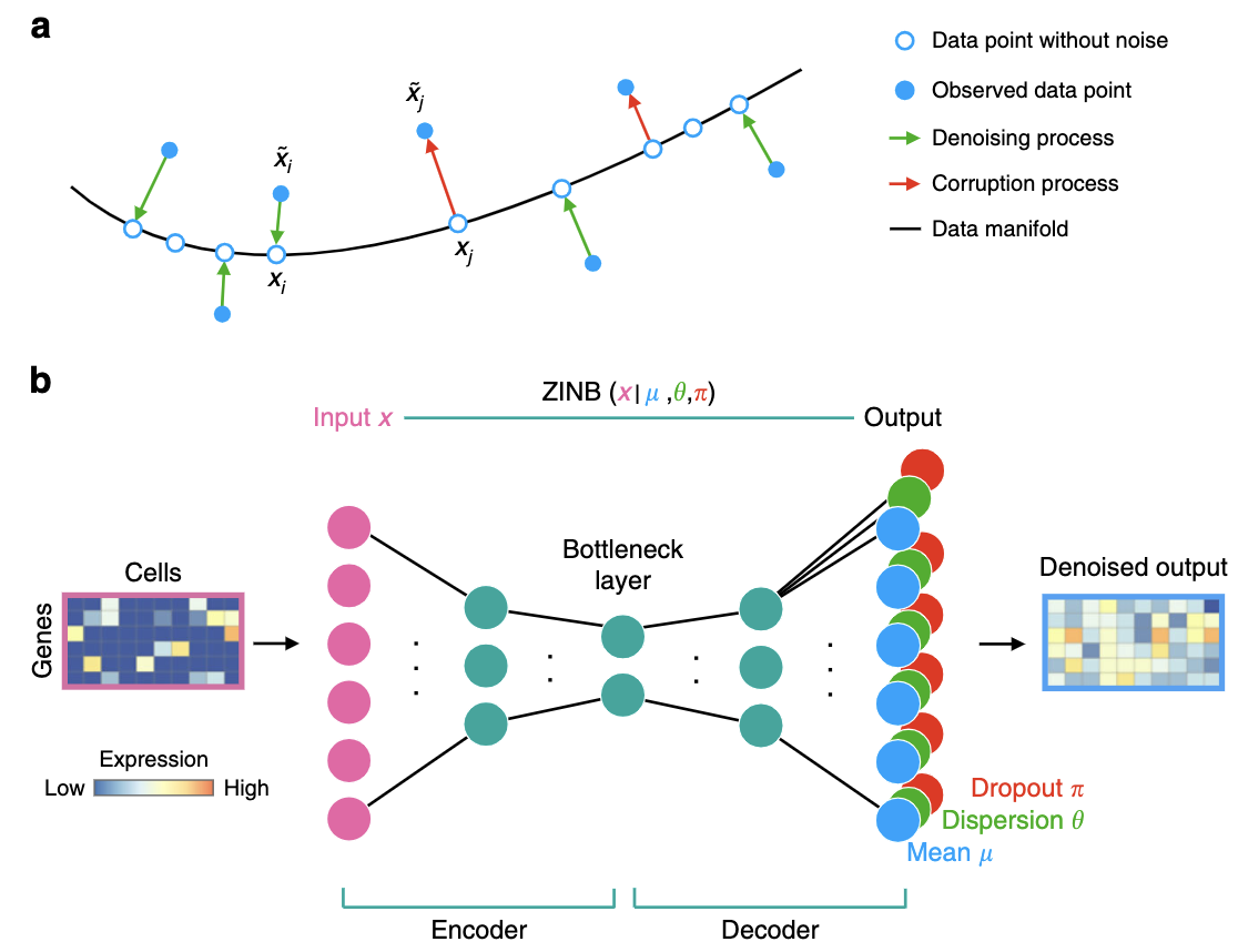
scVI (single-cell Variational Inference) is a specialized implementation of a Variational Autoencoder (VAE) tailored to single-cell RNA-seq data. It models the observed count data as being drawn from a negative binomial (NB) distribution, allowing it to account for the overdispersion inherent in single-cell data. The framework is designed to simultaneously capture the low-dimensional latent structure of the data and model the technical variability associated with sequencing, such as differences in library sizes.
Like a generic VAE, scVI consists of an encoder and a decoder. The encoder maps the observed gene expression counts ( X ) into a latent space ( Z ), capturing the underlying biological variation. The decoder reconstructs the counts ( X ) from ( Z ), but in scVI, this reconstruction explicitly models count data using the negative binomial distribution: [ X_{ij} (, r_j), ] where (* ) is the mean expression for gene ( j ) in cell ( i ), and ( r_j ) is the dispersion parameter for cell ( i ).
The latent space ( Z ) represents a compressed, biologically meaningful representation of each cell, and it is regularized to follow a standard Gaussian prior ( p(Z) = (0, I) ). The overall loss function to be minimized is the evidence lower bound (ELBO): \[ \begin{align*} \mathcal{L}(\text{encoder}, \text{decoder}; X_{1:n}) &= \sum_{i=1}^{n}\bigg[-\mathbb{E}_{q_{\text{encoders}}(Z_i, \ell_i \mid X_i)} \Big[ \log p_{\text{decoder}}(X_i \mid Z_i, \ell_i) \Big] \\ &\quad + \text{KL}\Big(q_{\text{encoder1}}(Z_i \mid X_i) \, \| \, p_{\text{prior1}}(Z_i)\Big) \\ &\quad + \text{KL}\Big(q_{\text{encoder2}}(\ell_i \mid X_i) \, \| \, p_{\text{prior2}}(\ell_i)\Big)\bigg], \end{align*} \]
where ( _i ) represents the library size (total counts per cell).
5.5.3 Architecture for library size and overdispersion
The architecture consists of:
Encoders: The input is the raw count \(X_i\). There are technically two encoders — one encodes the latent space \(Z_i\) (which represents the biological variation in cells) and the other, the library size \(\ell_i\). The first encoder, \(q_{\text{encoder1}}(Z_i \mid X_i)\), learns a multivariate Gaussian with a diagonal covariance matrix, and the second encoder, \(q_{\text{encoder2}}(\ell_i \mid X_i)\), is a log-normal distribution.
Decoder: The inputs are the latent variables \(Z_i\) and library size \(\ell_i\). The decoder predicts the mean \(\mu_{ij}\) for each gene \(j\) based on \(Z_i\), and \(\mu_{ij}\) alongside \(\ell_i\) are used to compute the objective function. (The dispersion parameter \(r_j\) is learned via variational Bayesian inference — see the paper.)
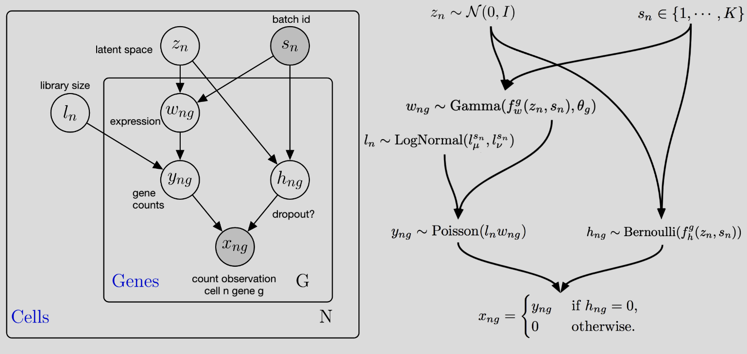
The so-called “plate diagram” in Figure 5.22 gives a good schematic summary of this architecture (but I’ve personally found that these diagrams are more of a “useful reminder” — they’re a bit hard to learn from directly).
5.6 Multi-modal integration (applicable beyond CITE-seq)
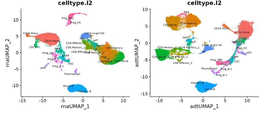
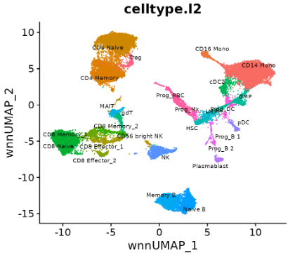
Coming back to CITE-seq data Section 5.4, suppose we have the following goal — we want to create a unified low-dimensional embedding (i.e., a “map” or “atlas” of sorts) that integrates the information from both the transcriptome and proteome. That is, there are some cell-type variations present only in the RNA or only in the ADT (Antibody-Derived Tags)10, and we want to create one unified embedding that combines all these information together. See Figure 5.23 and Figure 5.24 as an example.
Your first thought might be to simply perform PCA on the entire single-cell sequencing (i.e., one big PCA on all the 2000+ highly variable genes, and 100-ish proteins). However, this might not work as you might hope, since this wouldn’t account for the different scales and sparsities of RNA and ADT signals. That is, the RNA-dominated gene expression data could overwhelm the smaller protein feature set. This addresses the core challenge in simply combining modalities — differences in dimensionality, normalization, and noise — so that a single embedding captures both transcriptomic and proteomic variation while preserving each modality’s unique biological signal.
We will mention this concept of integration between two omics more in Section 6.6 when we talk about 10x multiome (RNA & ATAC). For now though, we will focus on TotalVI, which is one of the most common ways to achieve this goal for CITE-seq data.
5.6.1 TotalVI (and other methods for the “union” of information)
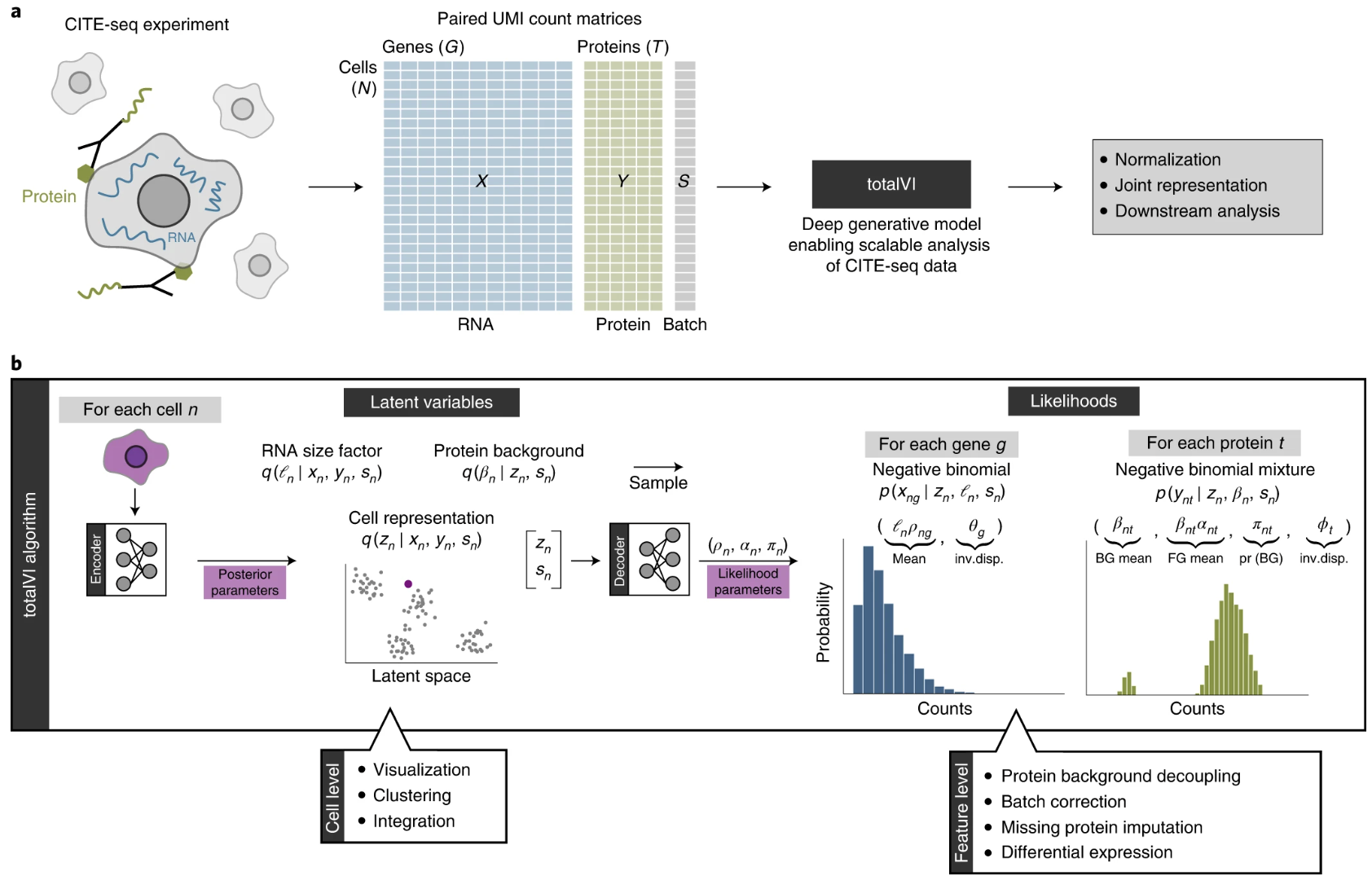
Input/Output. The input to TotalVI is a multi-modal sequencing matrix, where 1) the count matrix (for gene expression) \(X \in \mathbb{Z}_+^{n\times p}\) for \(n\) cells and \(p\) genes, and 2) the count matrix (for protein abundance) \(Y \in \mathbb{Z}_+^{n\times q}\) for \(n\) cells and \(q\) proteins. The output is: 1) \(Z \in \mathbb{R}^{n \times k}\), where \(k \ll \min\{p,q\}\) (where there are \(k\) latent dimensions), and also 2) the normalized gene expression matrix \(X' \in \mathbb{R}^{n\times p}\), and 3) the normalized protein abundance matrix \(Y' \in \mathbb{R}^{n\times q}\).
TotalVI (gayoso2021joint?) is a deep generative model specifically designed for the joint analysis of single-cell RNA and protein data obtained from techniques like CITE-seq. Unlike traditional single-cell RNA-seq methods that analyze transcriptomic data in isolation, TotalVI simultaneously incorporates transcriptomic and proteomic information to create a unified representation of cell states.
TotalVI builds upon the VAE framework of scVI, adapting it to the multimodal nature of CITE-seq data. The RNA counts are modeled with a negative binomial distribution, as in scVI, to capture overdispersion in single-cell data. For proteins, TotalVI introduces a mixture model that separates background and foreground components. This enables accurate modeling of protein measurements, even in the presence of high background noise. TotalVI’s decoder uses neural networks to predict the parameters of both the RNA and protein likelihoods, while the encoder maps cells into a shared low-dimensional latent space that reflects their joint transcriptomic and proteomic profiles. See Figure 5.25 for an overview.
5.6.1.1 The TotalVI model and key equations
TotalVI models RNA and protein counts \(x_{ng}\) and \(y_{nt}\) for gene \(g\) and protein \(t\) in cell \(n\) as follows:
\[ x_{ij} \sim \text{NB}(\ell_i \rho_{ij}, \theta_g), \quad \text{and}\quad y_{it} \sim \text{NB-Mixture}(\text{Foreground} + \text{Background}). \]
First, the RNA side: - \(\ell_n\): RNA library size for cell \(n\). - \(\rho_{ng}\): Normalized RNA expression frequency, predicted by the decoder network from the latent variables. - \(\theta_g\): Gene-specific overdispersion parameter for gene \(g\) (estimated for each gene during training, much like in scVI).
The values in \(\rho_{ng}\) are dictated by the learned latent embedding \(z_n\) using an encoder. A separate encoder will learn \(\ell_n\).
Next, the Protein side. The protein counts \(y_{it}\) are modeled with a negative binomial mixture:
\[ y_{nt} \sim v_{nt} \,\text{NB}(\beta_{nt}, \phi_t) + (1 - v_{nt}) \,\text{NB}(\alpha_{nt} \beta_{nt}, \phi_t), \]
where: - \(v_{nt}\): Bernoulli variable indicating whether the count is from the background or foreground. - \(\beta_{nt}\): Protein background mean, learned during training. - \(\alpha_{nt}\): Scaling factor for foreground counts. - \(\phi_t\): Protein-specific overdispersion parameter.
The values in \(v_{nt}\) and \(\alpha_{nt}\) (but not \(\beta_{nt}\)) are dictated by the latent embedding \(z_n\)11.
The latent embedding12 \(z_n \in \mathbb{R}^k\) dictates: 1. \(\rho_{ng}\) (normalized gene expression), 2. \(\alpha_{nt}\) (protein foreground counts), and 3. \(\phi_t\) (probability of the protein displaying a foreground count).

Now we understand the generative model (decoder). The encoder is composed of three separate encoders: 1. Encoding observed gene expression \(x_n\) and protein expression \(y_n\) to yield \(z_n\), 2. Encoding just \(x_n\) to yield \(\ell_n\), and 3. Encoding just \(y_n\) to yield \(\beta_n\).
The objective function is the evidence lower bound (ELBO) to be minimized:
\[ \begin{aligned} \mathcal{L}(\text{encoders}, \text{decoders}; x_{\text{all cells}}, y_{\text{all cells}}) &= \sum_{n} \bigg[-\mathbb{E}_{q_{\text{encoders}}(z_n, \ell_n, \beta_n | x_n, y_n)} \log p_{\text{decoders}}(x_n, y_n | z_n, \ell_n, \beta_n) \\ &\quad + \text{KL}\big(q_{\text{encoder1}}(z_n | x_n, y_n) \, \| \, p_{\text{prior1}}(z_n)\big) \\ &\quad + \text{KL}\big(q_{\text{encoder2}}(\ell_n | x_n) \, \| \, p_{\text{prior2}}(\ell_n)\big) \\ &\quad + \text{KL}\big(q_{\text{encoder3}}(\beta_n | y_n) \, \| \, p_{\text{prior3}}(\beta_n)\big) \bigg]. \end{aligned} \]
Remark 5.2. Why did I call these “union” methods?
From the generative model
\[ p_{\text{decoders}}(x_n, y_n | z_n, \ell_n, \beta_n) \]
the latent embedding \(z_n\) is used to generate both the RNA \(x_n\) and protein \(y_n\). Intuitively, \(z_n\) likely contains more information than either \(x_n\) or \(y_n\) alone. The goal of TotalVI is to create one big atlas that provides a bird’s-eye view of all the sources of variation in the data — some originating from RNA, others from protein.
A brief note on other approaches.
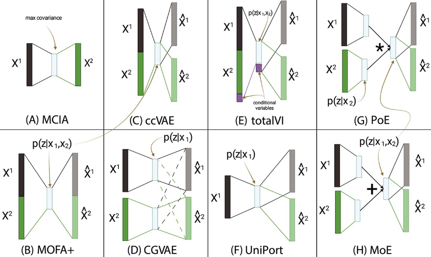
A popular non-deep-learning approach is Weighted Nearest Neighbors (WNN) (Hao et al. 2021) (shown in Figure 5.23 and Figure 5.24). More generally, methods for joint embeddings of multimodal data are discussed in (wang2024progress?), (brombacher2022performance?), and (makrodimitris2024depth?). Deep learning dominates this field, with differences in how architectures and losses manage information flow. See Figure 5.27.
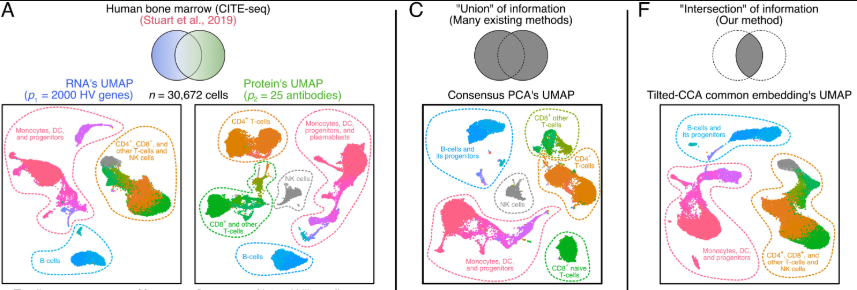
5.6.2 Correlation-based methods (i.e., “Intersection” of information)
Conceptually, you might appreciate that many of the methods described in Section 5.6.1 are about the “union” of information, in the sense that you’re trying to learn one singular embedding that could generate either modality, recall Remark 5.2. However, what if you wanted to learn what is the coordination between RNA and the cell surface markers? (That is, what if you don’t care there’s a lot of information unique to the cell surface markers – you instead want to just focus on what aspects of the RNA can be recapitulated in the cell surface markers?) This is where we might instead re-envision the goal of the embedding entirely and consider methods such as Tilted-CCA ((lin2023quantifying?), see Figure 5.28).
A brief review of CCA, to motivate Tilted-CCA.
The goal of Canonical Correlation Analysis (CCA) in data analysis is to identify and quantify the shared variation between two datasets by finding linear combinations of variables in each dataset that are maximally correlated, thereby revealing underlying relationships and shared structures across different data modalities.
Input/Output. The input of CCA is two matrices, \(X \in \mathbb{R}^{n \times p}\) and \(Y \in \mathbb{R}^{n \times q}\) be two datasets measured on the same \(n\) observations. The main output is \(Z^{(1)}, Z^{(2)} \in \mathbb{R}^{n \times k}\), where \(k \ll \min\{p,q\}\) (where there are \(k\) latent dimensions), which are the pair of canonical score matrices. Each pair of columns from \(Z^{(1)}\) and \(Z^{(2)}\) (for example, the first column of \(Z^{(1)}\) and the first column of \(Z^{(2)}\)) denote linear transformations (one applied to \(X\), another applied to \(Y\)) the yields the highest correlation possible.
Some brief description of the details: CCA seeks to identify linear projections of \(X\) and \(Y\) that are maximally correlated. Specifically, it finds vectors \(u \in \mathbb{R}^{p}\) and \(v \in \mathbb{R}^{q}\) that maximize the correlation between the canonical variables \(Xu\) and \(Yv\): \[ \max_{u, v} \quad \frac{u^\top \Sigma_{XY} v}{\sqrt{u^\top \Sigma_{XX} u} \sqrt{v^\top \Sigma_{YY} v}}, \quad \text{such that}\quad \|u\|_2 = \|v\|_2 = 1, \] where \(\Sigma_{XX}\), \(\Sigma_{YY}\), and \(\Sigma_{XY}\) are the covariance matrices of \(X\), \(Y\), and their cross-covariance, respectively. The solutions, known as , form the matrices \(Z^{(1)} = Xu \in \mathbb{R}^{n\times 1}\) and \(Z^{(2)} = Yv \in \mathbb{R}^{n\times 1}\), where \(u\) and \(v\) contain the canonical weights (“loadings”). This is for the first pair of canonical scores. To find the next pair of canonical scores, you perform the same optimization above but constrained that the next \(u\) and \(v\) are orthogonal to any of the preceding’s \(\{u,v\}\) pair of canonical scores. CCA is widely used for multimodal data integration, where it helps uncover shared structures between datasets by aligning their latent representations13. The solution for this is based on a series of eigen-decompositions of \(\Sigma_{XX}\), \(\Sigma_{YY}\), and \(\Sigma_{XY}\).
5.6.3 Brief description of Tilted-CCA
Tilted-CCA is a bit convoluted to explain mathematically, but the goal is self-contained.
Input/Output. The input to Tilted-CCA is any multi-modal sequencing matrix: the normalized matrix \(X \in \mathbb{R}^{n\times p}\) for \(n\) cells and \(p\) features, and another normalized matrix \(Y \in \mathbb{R}^{n\times q}\) for \(n\) cells and \(q\) features, where, importantly, 1) the two matrices need to be already preprocessed and normalized, and 2) the same \(n\) cells are measured in \(X\) and \(Y\) (i.e., paired data). The output is: \(C, D^{(1)}, D^{(2)} \in \mathbb{R}^{n \times k}\), where \(k \ll \min\{p,q\}\) (where there are \(k\) latent dimensions). Here, \(C\) denotes the “common” signal between \(X\) and \(Y\), while \(D^{(1)}\) and \(D^{(2)}\) denote the “modality-distinct” signal in only \(X\) but not \(Y\) (or vice versa, respectively). (Tilted-CCA can also output the “common” or “distinct” component of \(X\) or \(Y\).)
It’s easier to describe why a method like Tilted-CCA exists: CCA gives you two matrices (\(Z^{(1)}\) and \(Z^{(2)}\)). Tilted-CCA aims to decompose \(Z^{(1)}\) and \(Z^{(2)}\) into three matrices, one for the common signal between \(X\) and \(Y\), and the two others for the unique signals in each modality. Essentially, Tilted-CCA defines the “signal” via geometric relations based on the nearest-neighbor graph of cells. It does the following four-step process:
- Perform CCA: Perform CCA on \(X\) and \(Y\) to obtain the two canonical score matrices, \(Z^{(1)}\) and \(Z^{(2)}\).
- Learn the nearest-neighbor graphs: Construct the nearest-neighbor graphs, one based on the leading principal components of \(X\), and another based on the leading principal components of \(Y\). This yields two graphs, \(G^{(1)}\) and \(G^{(2)}\) (among the \(n\) cells).
- Construct the common nearest-neighbor graph: Based on \(G^{(1)}\) and \(G^{(2)}\), construct \(G\) which denotes the common geometric patterns found in both \(X\) and \(Y\).
- Decompose the canonical scores: Based on \(Z^{(1)}\) and \(Z^{(2)}\) and the common graph \(G\), learn a decomposition \(Z^{(1)} = C+D^{(1)}\) and \(Z^{(2)} = C+D^{(2)}\), where:
- \(C\) contains the common geometric relations found in \(G\), and
- \(D^{(1)}\) and \(D^{(2)}\) are orthogonal.
- \(C\) contains the common geometric relations found in \(G\), and
A brief note on other approaches.
There aren’t too many methods in this category for single-cell analyses yet, but it’s very common in broader computer science. CLIP (radford2021learning?) is a great example, where the goal is to learn how to jointly embed text and images, based on training data where each image has a caption. In the single-cell world, this task is sometimes called translation (not to be confused with the biological process of translation where mRNA gets translated into proteins). Here, “translation” means, “I want to translate the gene expression profile into the profile of a different modality.” BABEL (Wu et al. 2021) is an example of this (but this is for RNA-ATAC data, which is the omic we will be discussing next chapter in Chapter 6.)
Remark 5.3. Personal opinion: How do I tell if a multi-omic integration is doing the “union” or “intersection” of information?
Suppose you have paired multi-omic data (like in CITE-seq), and you are thinking of creating an embedding that puts each cell into one low-dimensional space, using both modalities. How do you tell if your planned method is the “union” (like in Section 5.6.1) or the “intersection” (like in Section 5.6.2)?
Broadly speaking, you want to ask yourself this loose conceptual question: Is your output embedding trying to preserve and aggregate all the biological signal across both modalities (i.e., envision a hoarder — someone not willing to let any biological information get thrown out), like in Total-VI? In that case, your method is more like a “union of information,” where you’re hoping to create one embedding that shows you “the best of both worlds” — regardless of which modality the signal is coming from, you want it in your embedding.
However, if your output embedding is purposefully trying to throw out biological signal such that the only signal remaining is specifically the ones that are shared between both modalities (i.e., envision the captain of a ship who wants the ship to go faster — someone willing to jettison anything overboard not essential), like in Tilted-CCA? In that case, your method is more like an “intersection of information,” where you’re hoping to only preserve the biological processes that affect both modalities. (If a process is specific to only the RNA and not the other omic, you don’t mind throwing it out because it might not be relevant to your question of interest.)
In the end, it’s all about the biology. What are you trying to understand from your data?
If you are interested in the math, there are actually a lot of matrix decompositions of multi-modal data, but each does something slightly different. My dichotomy of “union” and “intersection” is (in reality) overly simplistic. If you read into other matrix factorizations for multi-modal data, such as JIVE (lock2013joint?), you’ll need to think deeply about: 1) what the optimization problem is solving, and 2) how the optimization problem relates to the intended biology you’re trying to learn.
5.7 Note about the future: Intracellular proteins
Single-cell RNA sequencing (scRNA-seq) and multimodal techniques such as CITE-seq have revolutionized our ability to profile cellular states, but they remain largely focused on transcriptomic and surface protein measurements. Measuring single-cell proteomics presents unique challenges compared to single-cell RNA sequencing (scRNA-seq), largely due to the fundamental differences in how proteins and nucleic acids are analyzed. Unlike RNA, which can be amplified exponentially using PCR, proteins cannot be amplified in a similar manner. This makes every step of protein analysis — cell lysis, protein extraction, digestion, and mass spectrometry detection — subject to losses that can’t be recovered or compensated for by amplification. Additionally, most single-cell proteomic methods rely on well-characterized affinity reagents, typically antibodies, which come with limitations such as cross-reactivity and restricted target availability. Expanding the repertoire of affinity reagents, including recombinant antibody fragments and aptamers, is an ongoing effort to improve detection coverage and specificity. However, the need for high-quality reagents and complex conjugation strategies further complicates single-cell proteomics compared to the relatively straightforward barcoding and sequencing of mRNA. See (bennett2023single?) for a comprehensive review.
Recent technological advances are making intracellular protein sequencing feasible. Methods such as NEAT-seq (chen2022neat?) and intranuclear CITE-seq (chung2021joint?) are extending antibody-based oligonucleotide tagging to nuclear proteins, enabling the simultaneous measurement of chromatin accessibility, RNA expression, and transcription factor abundance. These approaches help bridge the gap between transcriptional and proteomic data by directly quantifying regulatory proteins at the single-cell level. Additionally, mass spectrometry-based single-cell proteomics (scMS) is emerging as an alternative that does not rely on affinity reagents, allowing for unbiased proteomic profiling, including the identification of post-translational modifications.
Looking ahead, efforts to integrate intracellular protein sequencing with existing multiomic platforms will likely transform our understanding of cellular regulation. This is often done by combining mass spectrometry with sequencing-based techniques, such as nanoSPLITS (fulcher2024parallel?), which enables parallel scRNA-seq and scMS from the same cell.
(When we discuss spatial proteomics briefly along spatial transcriptomics later in the notes in ?sec-chapter_9. See (mund2022unbiased?).)
6 Single-cell epigenetics
6.1 Primer on the genome, epigenetics, and enhancers
The genome is the complete set of DNA within an organism, encoding the instructions for life. While every cell in an organism typically contains the same genome, different cells exhibit distinct phenotypes and functions. This diversity arises not from changes in the underlying DNA sequence but from epigenetic regulation — heritable modifications that influence gene expression without altering the DNA itself. Epigenetics includes processes like DNA methylation, histone modification, and chromatin accessibility, all of which contribute to the dynamic regulation of gene activity in response to developmental cues and environmental signals.
Enhancers play a critical role in this regulatory landscape. These are DNA sequences that, while not coding for proteins themselves, can dramatically increase the transcription of target genes. Enhancers act by binding specific transcription factors, proteins that recognize and attach to DNA sequences to regulate gene expression. Some transcription factors require assistance from chaperone proteins, which ensure their proper folding and functionality, or pioneer proteins, which can access and open tightly packed chromatin to allow other factors to bind. This interplay highlights the complexity of the regulatory machinery that governs cellular function. See ?fig-enhancer-promoter to appreciate how complex this machinery is.
Proteins typically degrade much slower than mRNA fragments. See https://book.bionumbers.org/how-fast-do-rnas-and-proteins-degrade. For this reason, you might hypothesize that “cellular memory” is stored via proteins, not mRNA.↩︎
See https://www.youtube.com/watch?v=P_fHJIYENdI for a fun YouTube video for more about this.↩︎
Each feature in the protein modality in CITE-seq data is often called ADT. It might sometimes be called a protein marker as well.↩︎
Notice there is no “library size” for protein.↩︎
Each feature in the protein modality in CITE-seq data is often called ADT. It might sometimes be called a protein marker as well.↩︎
Notice there is no “library size” for protein.↩︎
Technically, \(z_n\) is a Logistic Normal, which means it’s a distribution over the simplex. See more details in https://docs.scvi-tools.org/en/latest/user_guide/models/totalvi.html.↩︎
It’s not too important to understand what this means, but you can see (kingma2019introduction?) for a formal definition.↩︎
Some details about this “complicated math”: The MAP is generally intractable to compute due to a very annoying normalization constant. So instead of computing MAP directly, we maximize the ELBO, which is a lower-bound of the likelihood. This is really the same trick used in deriving the EM algorithm. See https://towardsdatascience.com/bayesian-inference-problem-mcmc-and-variational-inference-25a8aa9bce29 or (Lotfollahi, Wolf, and Theis 2019) for a derivation of the ELBO, and (kingma2013auto?) for the formal objective function.↩︎
Each feature in the protein modality in CITE-seq data is often called ADT. It might sometimes be called a protein marker as well.↩︎
Notice there is no “library size” for protein.↩︎
Technically, \(z_n\) is a Logistic Normal, which means it’s a distribution over the simplex. See more details in https://docs.scvi-tools.org/en/latest/user_guide/models/totalvi.html.↩︎
Each feature in the protein modality in CITE-seq data is often called ADT. It might sometimes be called a protein marker as well.↩︎