3 Single-cell sequencing
Overivew of single-cell sequencing data
3.1 The sparse count matrix and the negative binomial
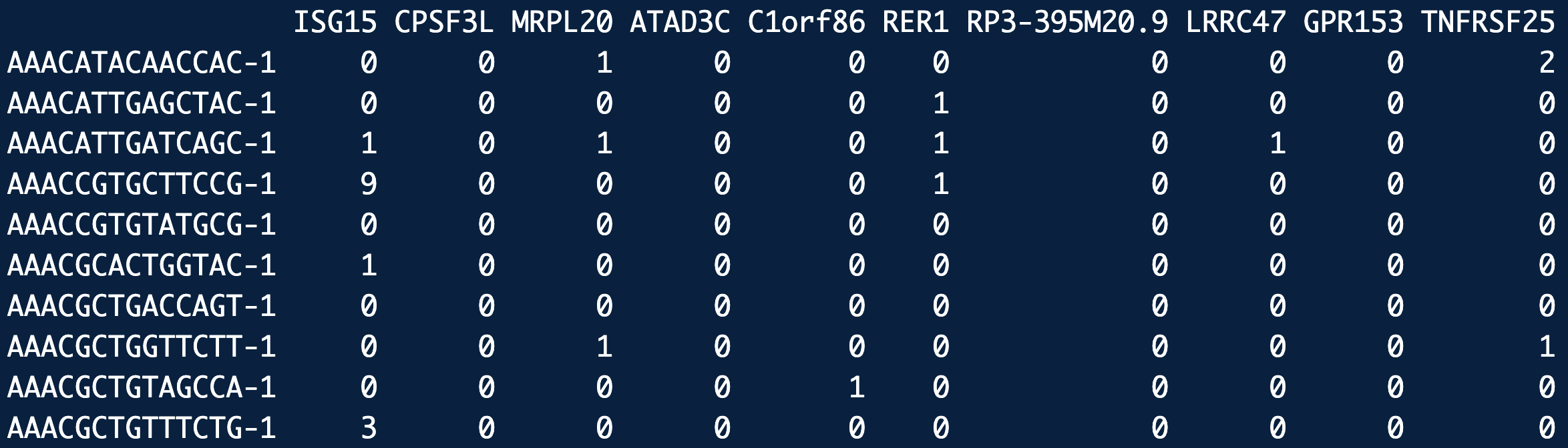
At the heart of single-cell sequencing data lies the sparse count matrix, where rows represent genes, columns represent cells, and entries capture the number of sequencing reads (or molecules) detected for each gene in each cell. This matrix is typically sparse because most genes are not expressed in any given cell, leading to a prevalence of zeros. The data’s sparsity reflects both the biological reality of selective gene expression and technical limitations such as sequencing depth. To model the variability in these counts, the negative binomial distribution is often employed. This distribution accommodates overdispersion, where the observed variability in gene expression counts exceeds what would be expected under simpler models like the Poisson distribution. By accounting for both biological heterogeneity and technical noise, the negative binomial provides a robust framework for analyzing sparse single-cell data.
Let \(X \in \mathbb{R}^{n\times p}\) denote the single-cell data matrix with \(n\) cells (rows) and \(p\) features (columns). In a single-cell RNA-seq data matrix, the \(p\) features represent the \(p\) genes.
Here are some basic statistics about these matrices (based mainly from my experience):
- For \(n\), we usually have 10,000 to 500,000 cells. These cells originate from a specific set of samples/donors/organisms1. See Figure 3.4 and Figure 3.5 for larger examples of single-cell datasets.
- For \(p\), we usually have about 30,000 genes (but as you’ll see, we usually limit the analysis to 2000 to 5000 genes chosen from this full set).2
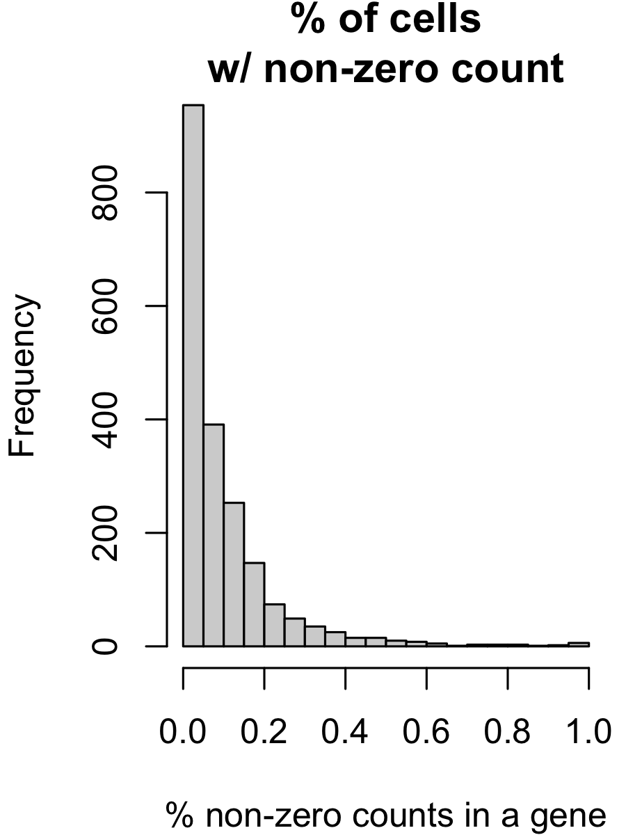
- In a typical scRNA-seq matrix, more than 70% of the elements are exactly 0. (And among the remaining 30%, typically half are exactly 1. The maximum count can be in the hundreds, i.e., the distribution is extremely right-skewed.) This is illustrated in Figure 3.1 and Figure 3.2. We’ll see later in ?sec-scrnaseq_tech where these “counts” come from.
Based on these observations, the negative binomial distribution is very commonly used.
The negative binomial (NB) distribution is a widely used model in single-cell RNA-seq analysis due to its ability to handle overdispersion, which is common in gene expression data. Overdispersion occurs when the variance of the data exceeds the mean, a phenomenon that cannot be captured by the Poisson distribution. The NB distribution introduces an additional parameter to model this extra variability, making it more flexible for single-cell data.
Let us focus on the count for cell \(i\) and gene \(j\), i.e., the value \(X_{ij}\). The probability mass function (pmf) of the NB distribution for a random variable ( X_{ij} ) is given by:
\[ P(X_{ij} = k) = \binom{k + r_j - 1}{k} p_{ij}^r (1 - p_{ij})^k, \quad k = 0, 1, 2, \ldots \tag{3.1}\]
where \(r_j \> 0\) is the dispersion (or “overdispersion”) parameter and \(p\_{ij} \in (0, 1)\) is the probability of success. This is the “standard” parameterization, mentioned in https://en.wikipedia.org/wiki/Negative_binomial_distribution. This specific parameterization is actually not very commonly used.
Alternatively, the NB distribution is most commonly parameterized in terms of the mean \(\mu_{ij}\) and the dispersion parameter \(r_j\), which is often preferred in single-cell analysis:
\[ \text{Mean: } \mu_{ij}, \quad \text{Variance: } \mu_{ij} + \frac{\mu_{ij}^2}{r_j} = \mu_{ij}\left(1 + \frac{\mu_{ij}}{r_j}\right). \tag{3.2}\]
(Compare these relations to the Poisson distribution, where both the mean and variance would be \(\mu_{ij}\).)
To relate equation Equation 3.1 to Equation 3.2, observe that we can derive,
\[ \mu_{ij} = \frac{r_j (1 - p_{ij})}{p_{ij}}. \]
We typically use a different overdispersion parameter \(r_j\) for each gene \(j \in \{1,\ldots,p\}\). Here, \(r_j\) controls the degree of overdispersion. When \(r_j \to \infty\), the variance approaches the mean, and the NB distribution converges to the Poisson distribution. For single-cell RNA-seq data, the introduction of \(r_j\) allows the model to capture both the biological variability between cells and technical noise, making it robust to the sparse and overdispersed nature of gene expression data.
Why would genes even have different overdispersions? We’re assuming in most statistical models that: 1) genes are modeled as a negative binomial random variable, and 2) genes have different overdispersion parameters \(r_j\). Why is this reasonable? Is there a biomolecular reason for this?
We draw upon Sarkar and Stephens (2021), explaining how the NB distribution is justified (both theoretically and empirically) for scRNA-seq data. After reading this paper, you’ll see that the overdispersion originates from the “biological noise” (i.e., the Gamma distribution). This differs from gene to gene because gene expression is subject to many aspects: transcriptomic bursting, the proximity between the gene and the promoter, the mRNA stability and degradation, copy number variation, the cell cycle stage, etc.
3.1.0.1 How do you estimate the overdispersion parameter in practice?
The easiest way is to use MASS::glm.nb in R. However, this is very noisy for single-cell data (see Remark 3.1). Since we are estimate one dispersion parameter per gene, many methods use an Empirical Bayes framework to “smooth” the overdispersion parameters (Love, Huber, and Anders 2014). More sophisticated methods (such as SCTransform (Hafemeister and Satija 2019)) use the Bioconductor R package called glmGamPoi. Deep-learning methods simply incorporate estimating the dispersion parameter into the architecture and objective function, see scVI (Lopez et al. 2018).
Also, note that which we are assuming here that the overdispersion parameter \(r_j\) is shared across all the cells for gene \(j\), there are methods that also use different overdispersion parameters for different cell populations. See Chen et al. (2018) or the dispersion parameter in scVI (see https://docs.scvi-tools.org/en/stable/api/reference/scvi.model.SCVI.html#scvi.model.SCVI). In general, using different overdispersion parameters for the same gene across different cell populations is not common, so my suggestion is to: 1) have a diagnostic in mind on how would you know if need to use different overdispersion parameters for the same gene, and then 2) try analyzing the genes where each gene only has one overdispersion parameter and see if you have enough concrete evidence that such a model was too simplistic.
Personal opinion: My preferred parameterization The formulation Equation 3.2 by far is the most common way people write the NB distribution. We typically call \(r_j\) the “overdispersion” parameter, since the inclusion of \(r_j\) in our modeling is typically to denote that there is more variance than a Poisson. I personally don’t like it because I find it confusing that a larger \(r_j\) denotes a distribution with smaller variance. Hence, I usually write the variance as \(\mu_{ij}(1+\alpha_j \mu_{ij})\) (where \(\alpha_j = 1/r_j\)). This way, \(\alpha_j = 0\) is a Poisson distribution. However, even though this makes more sense to me, it’s not commonly used. (It’s because this parameterization makes it confusing to work with the exponential-family distributions mathematically.)
The main takeaway is to always pay close attention to each paper’s NB parameterization. You’re looking for the mean-variance relation written somewhere in the paper to ensure you understand the author’s notation.
Remark 3.1. What makes the negative binomial tricky Let me use an analogy that is based on the more familiar coin toss. Suppose 30 people each are given a weighted coin where the probability of heads is \(10^{-9}\) (basically, it’s impossible to get a heads). Everyone coerce and agree to a secret number \(N\), and everyone independently flips their own coin \(N\) times and records the number of heads. I (the moderator) do not know \(N\), but I get to see how many heads each person got during this experiment. My goal is to estimate \(N\). What makes this problem very difficult?
If \(N\) were 10, or 100, or maybe even 10,000, almost everyone would get 0 heads. That is, we cannot reliably estimate \(N\) since the log-likelihood function is very flat. The issue is because count data has a finite resolution — 0 is always the smallest possible value, and 1 is always the second smallest value. Hence, unlike continuous values (which have “infinite resolution” in some sense), non-negative integers “lose” information the smaller the range is.
Returning the negative binomials, consider a simple coding example:
set.seed(10)
mu <- 1
true_overdispersion <- 1000
true_size <- mu / (true_overdispersion - 1)
data <- stats::rnbinom(1e5, size = true_size, mu = mu)
overdispersion_vec <- exp(seq(log(1), log(1e7), length.out = 100))
log_likelihood <- sapply(overdispersion_vec, function(overdispersion) {
  size <- mu / (overdispersion - 1)
  sum(dnbinom(data, size = size, mu = mu, log = T))
})
hist(data,
     main = paste("% 0:", round(length(which(data == 0)) / length(data) * 100, 2),
                  "\nEmpirical mean:", round(mean(data), 2),
                  "\nEmpirical variance:", round(var(data), 2))
)
hist(data[data != 0])
plot(log10(overdispersion_vec), log_likelihood)
plot(log10(overdispersion_vec[-c(1:5)]), log_likelihood[-c(1:5)])
3.1.1 Remembering that these cells come from donors/tissues!
The \(n\) cells in our single-cell dataset originate from \(m\) tissues/samples/donors/etc. That is, the cells are stratified (or hierarchically organized). Based on your scientific question of interest, this is a consideration you might want your analysis to take into account. In general, each of the \(n\) cells in your single-cell dataset will have “metadata” (such as which sample the cell came from). See Figure 3.4 and Figure 3.5 as examples. We will see in Section 4.4.12 on how some methods explicitly take into account this “hierarchical” structure of the data. However, most methods that are intended for cell lines or genetically-controlled scenarios do not focus on this hierarchical structure (since all the cell-lines or organisms are nearly identical).


Typically, you can expect that the cells in a single-cell analysis come from one of three categories:
Cell-lines (In vitro): Cells grown in controlled laboratory conditions, such as HeLa or HEK293, typically on a petri dish, are commonly used for experiments requiring consistency and ease of manipulation. These cells are ideal for studying specific pathways or drug responses in a simplified system.
Model organisms (In vivo): Cells derived from model organisms (such as zebrafish, genetically engineered mice, yeast, specific plants, etc.) allow researchers to study conserved biological processes in a controlled, organismal context. These systems often provide genetic and developmental insights that are directly relevant to human biology.
Humans (In vivo): Cells from human tissues or blood samples provide direct insights into human biology, disease mechanisms, and patient-specific variability. They are often used in translational research to bridge findings from cell lines and model organisms to clinical applications.
Other categories, such as xenografts, organoids, and co-culture systems, also play critical roles in capturing specific aspects of cellular behavior and interactions.
3.2 The role of normalization to adjust for sequencing depth
Normalization is a critical step in the analysis of single-cell sequencing data, addressing the technical variability introduced by differences in sequencing depth across cells. Sequencing depth refers to the total number of reads obtained for each cell, which can vary due to technical factors like library preparation or instrument sensitivity. Without normalization, cells with higher sequencing depth might appear to express more genes simply because of greater read coverage, not biological differences. Normalization methods aim to make gene expression counts comparable across cells by adjusting for these differences, ensuring that downstream analyses reflect true biological variation rather than technical artifacts. This step is foundational for accurate clustering, differential expression analysis, and other interpretative tasks in single-cell studies.
It has been known for a long time that when dealing with count data, proper normalization is foundational to properly doing meaningful inference. See (Risso et al. 2014). As we will see in Chapter 3, sequencing technologies cannot control how many reads (i.e., “counts”) are sequenced from each cell – this depends on the biochemistry efficency. Also, larger cells typically have more reads (which is itself a confounder) (Maden et al. 2023). We will describe normalization in more detail in Section 3.3.6.
3.3 The typical workflow for any sc-seq data
We will now describe the common steps at the start of a single-cell sequencing computational workflow (i.e., the steps that happen after the data has been collected and been aggregated into a matrix). More details about the downstream steps will be discussed in detail in Chapter 3. See (Luecken and Theis 2019; Heumos et al. 2023) for fantastic tutorials on best practices (among many). I’ll like to plug my own paper about best practices (Prater and Lin 2024).

For additional reference: See https://www.sc-best-practices.org/ and https://www.bigbioinformatics.org/intro-to-scrnaseq.
3.3.1 (Optional) Ambient reads
(This step will make more sense once you know a bit about how scRNA-seq data is generated, see Chapter 3.)
Ambient reads and doublets (see Figure 3.7) are common technical artifacts in single-cell sequencing data that can distort biological interpretations if left unaddressed. Ambient reads arise from background RNA that is captured during sequencing but does not originate from the cell being analyzed. These reads can falsely inflate gene expression levels, particularly for highly abundant transcripts. Detecting and mitigating these artifacts is an optional but valuable step in data preprocessing, as it improves the overall quality and biological relevance of downstream analyses.

Input/Output. The input to ambient detection is a count matrix \(X\in \mathbb{Z}_+^{n\times p}\) for \(n\) cells and \(p\) features (i.e., genes), and the output is \(X'\in \mathbb{Z}_+^{n'\times p}\) where \(X'_{ij} \leq X_{ij}\) for all cell \(i\) and feature \(j\).
3.3.2 How to do this in practice
This is not always done in a standard analysis of 10x scRNA-seq data because the CellRanger pipeline does a pretty good job for you already by default. However, for certain finicky biological systems that deviate from the norm, you might purposely not use CellRanger’s default ambient detection and doublet detection, and instead choose to manually perform your own so that you have more control. In that case, the main ambient RNA detection method I’ve seen used is SoupX (Young and Behjati 2020).
3.3.3 Cell filtering (or doublet detection)
Cell filtering is a crucial preprocessing step in single-cell sequencing analysis, aimed at removing low-quality or irrelevant cells to ensure reliable downstream analyses. During the sequencing process, some cells may produce insufficient data due to poor capture efficiency, leading to low gene counts or incomplete profiles. Additionally, some “cells” may actually be empty droplets or doublets. Doublets occur when two cells are captured together in the same droplet or well, leading to mixed gene expression profiles that do not represent any single cell. Filtering typically involves setting thresholds on metrics like the total number of detected genes, the fraction of mitochondrial gene reads (a marker of stressed or dying cells), and overall sequencing depth. By carefully selecting cells that meet quality standards, researchers can reduce noise, improve the robustness of analyses, and focus on biologically meaningful signals. This step helps ensure that the dataset represents a true and interpretable snapshot of cellular diversity.
(Typically, ambient RNA means you’re trying to subtract “background” counts from your scRNA-seq matrix. The number of cells remains the same. In contrast, cell filtering is removing cells, typically geared to target cells deemed to be empty droplets or doublets.)
Input/Output. The input to cell filtering is a count matrix \(X\in \mathbb{Z}_+^{n\times p}\) for \(n\) cells and \(p\) genes, and the output is \(X'\in \mathbb{Z}_+^{n'\times p}\) where \(n' \leq n\), whose rows are a strict subset of those in \(X\).
3.3.4 How to do this in practice
This is commonly using the subset function in R, where we commonly filter based on nFeature_RNA (i.e., the number of genes that are expressed in a cell) and percent.mt (i.e., the fraction of counts that are originating from mitochondrial genes). The latter is usually computed using Seurat::PercentageFeatureSet3. See Figure 3.8 for an illustration. There is no commonly used threshold for these filters, but it typically depends on removing the extreme quantiles in your dataset. If this simple filter isn’t sophisticated enough to detect doublets (and you have good biological/technical reasons to suspect doublets, typically due to either the cell isolation or droplet formulation step), the doublet detection method I’ve seen used is DoubletFinder (McGinnis, Murrow, and Gartner 2019).
Note: In Seurat, the cells are denoted as columns and features (such as genes) as rows. This is the transpose of the typical statistical notation.

We usually filter based on nFeature_RNA because cells with too few genes are potentially deemed as empty droplets, and cells with too many genes are potentially deemed as doublets. High percentage of gene expression from mitochondrial genes is typically an indicator of poor sample quality4.
3.3.5 A brief note on other approaches
See (Xi and Li 2021) for a benchmarking of doublet detection methods.
3.3.6 Normalization
Normalization is a key step in single-cell sequencing analysis, designed to adjust raw data so that gene expression measurements are comparable across cells. Variability in sequencing depth and technical artifacts can cause discrepancies in the total number of reads captured per cell, making raw counts unsuitable for direct comparison. Normalization methods address this by scaling or transforming the data to account for these differences, ensuring that observed expression levels more accurately reflect true biological variation. Approaches can range from simple scaling based on total counts to more sophisticated strategies that model the underlying distribution of the data. Normalization not only improves the accuracy of downstream analyses, such as clustering and differential expression, but also enhances the interpretability of results by reducing technical noise.
Typically, the normalization has the following form:
\[ X_{ij} \leftarrow \log\Big(\frac{10,000 \cdot X_{ij}}{\sum_{j'=1}^{p}X_{ij'}}+1 \Big). \tag{3.3}\]
The fraction \(X_{ij}/\sum_{j'=1}^{p}X_{ij'}\) allows us to model the relative proportions (instead of absolute counts) of gene expression in each cell. The \(\log(\cdot)\) is to handle the right-skewed nature of the data (since an entry of \(X_{ij}\) is still 0 even after computing the fraction, and taking a fraction doesn’t adjust for the skewed nature by itself). The \(+1\) is handle the fact that we cannot take \(\log(0)\). The only arbitrary thing in the factor of 10,000 – it’s simply for convenience to scale all the values (remember, \(\log(AB) = \log(A) + \log(B)\), so essentially, this normalization is shifting all the fractions up by \(\log(10,000)\)). The number of 10,000 (or sometimes 1 million) became commonplace because we can now interpret the number \(10,000 \cdot (X_{ij}/\sum_{j'=1}^{p}X_{ij'})\) as the hypothetical number of counts we would’ve gotten in cell \(i\) for gene \(j\) if the sequencing depth of cell \(i\) were 10,000.
3.3.7 How to do this in practice
See the Seurat::LogNormalize function, illustrated in Figure 3.9.

Input/Output. The input to normalization is a count matrix \(X\in \mathbb{Z}_+^{n\times p}\) for \(n\) cells and \(p\) features (i.e., genes), and the output is \(X'\in \mathbb{R}^{n\times p}\).
3.3.8 A brief note on other approaches
There’s actually a lot of normalization methods since normalizing count data has existed ever since bulk-sequencing. However, three notable mentions are: SCTransform (Hafemeister and Satija 2019) which uses a NB GLM model to normalize data and GLM-PCA (Townes et al. 2019) which uses a GLM matrix factorization to adjust for sequencing depth, where both methods use adjust using the observed sequencing depth for each cell. Deep-learning methods like scVI (Lopez et al. 2018) include the library size as a latent variable to be estimated itself. See (Lause, Berens, and Kobak 2021; Ahlmann-Eltze and Huber 2023) for benchmarkings.
Remark (Personal opinion: The log-transformation and lack of the negative binomial). It is well documented that this log-normalization is not best – see (Townes et al. 2019) and (Hafemeister and Satija 2019) for in-depth discussions. The issues stem from “discrete-ness” of the log transformation. However, surprisingly, as shown in papers such as (Ahlmann-Eltze and Huber 2023), the log-transformation is actually quite robust.
3.3.9 Feature selection
Feature selection is a critical step in single-cell sequencing analysis that focuses on identifying the most informative genes for downstream analyses. Single-cell datasets often include thousands of genes, many of which may be uninformative due to low variability or consistent expression across all cells. By narrowing the focus to a subset of highly variable genes (HVGs), feature selection reduces noise, enhances computational efficiency, and highlights the genes most likely to drive biological differences. These selected features are used in clustering, dimensionality reduction, and other tasks where capturing meaningful variation is essential. Effective feature selection ensures that the resulting analyses are both interpretable and biologically relevant.
Input/Output. The input to feature selection is a count matrix \(X\in \mathbb{Z}_+^{n\times p}\) for \(n\) cells and \(p\) features (i.e., genes)5, and the output is \(X'\in \mathbb{R}^{n\times p'}\) where \(p' \leq p\), whose columns are a strict subset of those in \(X\).
3.3.10 The standard procedure: Variance Stabilizing Transformation
The vst (variance stabilizing transformation) procedure is a commonly used method in single-cell RNA-seq analysis for identifying highly variable genes. It is designed to account for the relationship between a gene’s mean expression and its variability, ensuring that variability is measured in a way that is independent of mean expression levels. The procedure involves the following steps:
- Fitting the Mean-Variance Relationship:
First, the relationship between the log-transformed variance and log-transformed mean of gene expression values is modeled using local polynomial regression, commonly referred to as loess. This step captures the expected variance for a given mean expression level. Let \(\mu_j\) denote the mean expression of gene \(j\) and \(\sigma_j^2\) its variance. The loess fit provides the expected variance, \(\hat{\sigma}_j^2\), as a smooth function of \(\log(\mu_j)\).
- Standardizing Gene Expression Values:
The observed expression values for each gene are then standardized to account for the expected variance: \[
Z_{ij} = \frac{X_{ij} - \mu_j}{\sqrt{\hat{\sigma}_j^2}},
\] where \(X_{ij}\) is the observed expression value for gene \(j\) in cell \(i\), \(\mu_j\) is the observed mean for gene \(j\), and \(\hat{\sigma}_j^2\) is the expected variance given by the fitted loess line. This standardization ensures that variability is measured relative to what is expected for genes with similar mean expression levels.
- Clipping and Variance Calculation: To prevent outliers from dominating the analysis, the standardized values \(Z_{ij}\) are clipped to a maximum value, determined by a parameter such as
clip.max. The variance of each gene is then calculated based on the clipped standardized values. Genes with the highest variance are selected as highly variable and prioritized for downstream analyses, such as clustering and trajectory inference.
This procedure addresses the inherent bias where genes with higher mean expression tend to exhibit greater variance, even if this variance is not biologically meaningful. By standardizing variability against the expected mean-variance relationship, the vst method provides a robust approach to identifying genes that truly capture biological heterogeneity across cells.
Remark (Feature selection, agnostic of the rest of the analysis). For the statistical students, feature selection might seem a bit odd. After all, we’re selecting the genes to use in our analysis (again, typically about 2000 genes among 30,000 genes) before we do any other modeling. This is unlike the Lasso, where the feature selection is done while we’re doing a downstream task (i.e., regression in this case).
In a scRNA-seq analysis, we typically use the HVGs upfront, and use only these genes for all remaining downstream analyses. This is mainly for pragmatic reasons – most genes are 0’s in almost all the cells, so there’s no need to involve these genes in any of our downstream analysis.
3.3.11 How to do this in practice
See the Seurat::FindVariableFeatures function, illustrated in Figure 3.10.

3.3.12 A brief note on other approaches
See (Zhao et al. 2024) for an overview of feature selection methods. This is a interesting statistical modeling question in the sense that the goal for these methods is often how to distinguish between “technical variance” (i.e., variation attributed to sequencing depth) from “biological variance” (i.e., if a gene has different expressions across cells in the tissue).
3.3.13 (Optional) Imputation
Imputation refers to methods used to infer missing or undetected values in single-cell sequencing data, particularly addressing the zeros that dominate scRNA-seq datasets. Early in the development of single-cell technologies, these zeros were often attributed to “dropouts,” where lowly expressed genes failed to be captured due to technical limitations. Zero-inflated models were developed to distinguish between “true” biological zeros – where a gene is genuinely not expressed – and dropout zeros, filling in the latter to provide a more complete representation of gene expression. However, with advancements like unique molecular identifiers (UMIs), scRNA-seq data have become more reliable and less prone to dropout artifacts. As a result, the need for imputation has diminished, and modern workflows often bypass it entirely, favoring raw or minimally processed data that more accurately reflect true biological variation. Imputation remains an optional step, typically reserved for specific analyses where reconstructing missing data is critical. See (Hou et al. 2020) for a review of many methods in this category.
See (Kharchenko, Silberstein, and Scadden 2014) for the landmark paper that originally discussed dropouts. However, see Remark 4.2 for why these “dropouts” are no longer common to worry about in your single-cell analysis.
3.3.14 How to do this in practice
I’ve see MAGIC (Markov Affinity-based Graph Imputation of Cells) (Van Dijk et al. 2018) used quite often, if there’s a data imputation being performed. This method imputes missing gene expression values by leveraging similarities among cells using a graph-based approach. MAGIC constructs a nearest-neighbor graph where cells are nodes, and edges represent biological similarity. Through data diffusion, information is shared across similar cells to denoise and recover underlying gene expression patterns. See Figure 3.11.

3.3.15 Dimension reduction
Dimension reduction, particularly methods like Principal Component Analysis (PCA) and Singular Value Decomposition (SVD), serves as a cornerstone in single-cell sequencing analysis. The primary goal is twofold: first, to obtain a low-dimensional representation of the data, which is critical for visualizing complex datasets and enabling computationally efficient downstream analyses such as clustering and trajectory inference. By condensing thousands of genes into a smaller number of principal components, researchers can focus on the dominant patterns of variation that drive biological differences. Second, dimension reduction helps denoise the data by filtering out technical noise and minor variations that are less biologically relevant. This makes the resulting analysis more robust and interpretable, allowing researchers to capture meaningful cellular heterogeneity while mitigating the impact of sparsity and noise inherent to single-cell datasets.
Input/Output. The input to dimension reduction is a matrix \(X\in \mathbb{R}^{n\times p}\) for \(n\) cells and \(p\) features (i.e., genes). The output is \(Z \in \mathbb{R}^{n\times k}\) where \(k \ll p\) (where there are \(k\) latent dimensions, typically between 5 to 50). We call \(Z\) the score matrix. Most dimension reduction (typically only linear ones – i.e., ones based on a matrix factorization) also return: (1) gene loading matrix \(W \in \mathbb{R}^{p \times k}\), and (2) “denoised” matrix \(X'\in \mathbb{R}^{n\times p}\), which is some form of \(X' = ZW^\top\).
3.3.16 The standard procedure: PCA
Principal Component Analysis (PCA) is a dimensionality reduction technique widely used in single-cell RNA-seq analysis to simplify complex datasets while retaining the most important patterns of variation. By transforming high-dimensional gene expression data into a smaller set of principal components, PCA captures the dominant trends in the data, such as differences between cell types or states. This reduced representation helps to mitigate the noise and sparsity inherent in single-cell data, making downstream tasks like clustering, trajectory inference, and visualization more efficient and interpretable. PCA serves as a foundational step in many single-cell workflows, offering both computational efficiency and biological insight.


I’ll describe the PCA in a bit more detail here since it’s can be a bit confusing.
Theorem (Equivalent formulations of PCA). Let \(X \in \mathbb{R}^{n\times p}\) be a centered matrix ( i.e., \(\overline{X}_{\cdot j} = 0\) for all \(j\in\{1,\ldots,p\}\)) and \(K\) be a pre-chosen latent dimensionality (such that \(k \ll p\)). Let \(\hat{\Sigma} = X^\top X/n\) denote the empircial covariance matrix.
The following four estimated embeddings \(\hat{Z} \in \mathbb{R}^{n\times k}\) are “equivalent.”
Maximization of information captured by the covariance (shown in Figure 3.12 (left)): Define \(\hat{Z} = X\hat{W}\) where \[ \hat{W} = \argmax_{W \in \mathbb{R}^{p\times K}}\tr\Big(W^\top \hat{\Sigma} W\Big), \quad \text{such that} \quad W^\top W = I_K. \tag{3.4}\]
Minimization of reconstruction error (via squared Euclidean loss) (shown in Figure 3.12 (left)): Define \(\hat{Z} = X \hat{W}\) where \[ \hat{W} = \argmin_{W \in \mathbb{R}^{p\times K}}\frac{1}{n}\sum_{i=1}^{n}\Big\|X_{i\cdot} - WW^\top X_{i\cdot}\Big\|^2_F \quad \text{such that} \quad W^\top W = I_K. \tag{3.5}\]
Low-rank approximation of the interpoint distances (via squared Euclidean distances): Let \(D_X \in \mathbb{R}^{n\times n}_+\) denote the matrix of squared Euclidean distances among all \(n\) samples in \(X\), i.e., \([D_X]_{i_1,i_2} = \|X_{i_1,\cdot} - X_{i_2,\cdot}\|^2_F\) for all \(i_1,i_2 \in \{1,\ldots,n\}\). (This is a function of \(X\).) Then, construct \(\hat{Z}=X\hat{W}\) where \[ \hat{W} = \argmin_{W \in \mathbb{R}^{p\times K}} \sum_{i_1,i_2 \in \{1,\ldots,n\}} \big[D_X\big]_{i_1,i_2} - \big[D_{XW}\big]_{i_1,i_2} \quad \text{such that} \quad W^\top W = I_K, \tag{3.6}\] and \(D_{XW} \in \mathbb{R}^{n\times n}_+\) is the matrix of squared Euclidean distances constructed from \(XW\).
Notice that Formulation #3 is simply the sum of differences (not squared) since projections are non-expansive, so the interpoint Euclidean distances necessarily decrease. We are not accurately describing the identifiability conditions above to formalize what “equivalence” technically means.
Some remarks:
- Relation to eigen-decompositions: PCA is fundamentally tied to eigen-decompositions due to the Low-Rank Approximation theorem6 (more formally, the Eckart-Young-Mirsky theorem). Specifically, \(\hat{W}\) is the eigenvalues of \(\hat{\Sigma}\), the covariance matrix. See Figure 3.13 (right).
(If you are familiar with how to manipulate eigen-decompositions, you can convince yourself that Formulation 2 is most directly related to the Low-Rank Approximation.)
- Interpretation of Formulation #1: In Formulation 1, we want to project the data \(X\) onto a lower-dimensional subspace defined by \(\hat{W}\) such the low-dimensional data \(\hat{Z}\) has as much variance as possible. This is by far the most common explanation of PCA. Part of its appeal is that it’s easy to explain what the “population model’s target quantity” is through this interpretation, but 1) it requires you to intrinsically understand why preserving covariance is something useful when we’re more interested in about the cells themselves, and 2) does not give insight to the more popular extensions of PCA.
Adjustable aspects to obtain other dimension-reduction methods: 1) Choosing a more suitable estimate of the population covariance \(\Sigma = \mathbb{E}[X^\top X]/n\) (or its correlation counterpart), or 2) enforcing additional structure (such as sparsity) onto the columns of \(\hat{W}\).
- Interpretation of Formulation #2: In Formulation 2, we want to project the data \(X\) onto a lower-dimensional subspace defined by \(\hat{W}\) such that the ambient-dimensional data is as close to the original data as possible (i.e., the projection “disturbs” the data the least). This interpretation reveals that PCA is trying to find the subspace that “distorts” each cell’s expression the least. While this won’t be used to motivate more modern embedding methods, it 1) offers a formal relation between PCA and matrix denoising, and 2) is the motivation for autoencoders later on.
Adjustable aspects to obtain other dimension-reduction methods: 1) How to measure the “error” between each cell’s expression and its reconstructed expression, 2) how this reconstruction is constructed given a cell’s low-dimensional representation?
- Interpretation of Formulation #3: In Formulation 3, we conceptually think about the cells’ interpoint distances (i.e., the distances between any two pairs of cells). Then, we want to project the data \(X\) onto a lower-dimensional subspace defined by \(\hat{W}\) such the low-dimensional data \(\hat{Z}\) preserves the distances between any two pairs of cells as much as possible. This perspective is perhaps the most intuitive, and also most revealing on the shortcomings of PCA. PCA is choosing to preserve the pairwise distances in a very specific fashion, via the squared Euclidean distances. There are a two aspects that reveal the deficiency of PCA:
- PCA is trying to preserve the squared Euclidean distance, so it’s going to put most of its attention on pairs of points that are very far away from one another.
- We consider all pairs of points.
These two aspects combined yield the qualitative statement that “PCA favors a global embedding that preserve far-away points”.7 In some sense, this is the exact opposite of what we want – qualitatively, we probably care more about getting the relative distances of each points and its immediate/local neighbors (so we can accurately see the subtle shifts in cells, as in trajectory inference).
Adjustable aspects to obtain other dimension-reduction methods: 1) How we’re measuring distance in \(X\) or in \(Z\) we’re using (perhaps using a distance that adapts to the geometry of the data), 2) how to measure the “distortion” in the pairwise distances, 3) which pairs of cells do we care about preserving their distances?
- References for the proofs: Relating one and two is mainly an exercise in matrix algebra. To show that Formulation #3 is also PCA, see Theorem 14.4.1 in (Kent, Bibby, and Mardia 1979).
Remark (The words we use to call the columns of \(\hat{W}\) after doing a linear-dimension reduction method like PCA). Note that \(\hat{W}\) is a \(p\)-by-\(K\) matrix. That is, each column of \(\hat{W}\) has one number for each feature (i.e., gene). We typically call each column one of a few things: “gene program” or “pathway” (both more biology-facing) or “eigen-gene” or “topic” (both more statistics-facing). Regardless, these words is to denote that each column of \(\hat{W}\) denotes a set of genes that work together, based on the magnitude and sign that feature has in this column.
3.3.17 How to do this in practice
See the Seurat::RunPCA function, illustrated in Figure 3.14. The resulting visualization is shown in Figure 3.15.


Seurat::DimPlot(pbmc, reduction = "pca") function to visualize the first two PCs. See the tutorial in https://satijalab.org/seurat/articles/pbmc3k_tutorial.html.
3.3.18 A brief note on other approaches
The distinction between “imputation” and “dimension reduction” gets murky because 1) computationally, many imputation methods rely on a dimension reduction, and 2) statistically, due to the low-rank approximation property of PCA, you can interpret many dimension reductions methods as an imputation method. When I say that “imputation is optional,” what I really mean is that modeling zero-inflation is typically optional.
Reviews of imputation methods such as (Hou et al. 2020) contain overview of dimension-reduction methods. eSVD (Lin, Qiu, and Roeder 2024) and GLM-PCA (Townes et al. 2019) are dimension reduction methods that leverage the fact that the NB is in the exponential family (among many). FastTopics (Carbonetto et al. 2021) is a popular non-negative matrix factorization method (among many) for modeling single-cell data. (We won’t have time to discuss non-negative matrix factorization in this course.) All these mentioned methods are able to perform normalization with dimension reduction simultaneously. Also, dimension-reductions are commonly folded into a method that aims to do multiple tasks simultaneously (for example, see scINSIGHT (Qian et al. 2022), among many examples). See (Ghojogh et al. 2021) for a massive review of common dimension-reduction frameworks.
However, by far the most popular method nowadays is using VAEs, since it is easy to combine dimension reduction with other downstream tasks. We’ll discuss VAEs in more detail in Section 5.5.2.
Remark (Personal opinion: Considerations for picking an appropriate dimension-reduction method). The categorizations of “linear” vs. “non-linear” is a bit blurry. Personally, I would call methods like eSVD (Lin, Qiu, and Roeder 2024) and GLM-PCA (Townes et al. 2019) as “linear” (in addition to PCA and fastTopics (Carbonetto et al. 2021)) since you estimate a matrix factorization and there’s a fixed transformation that relates the observed count \(X_{ij}\) to the inner product between a cell’s latent vector \(Z_{i,\cdot}\) and a gene’s latent vector \(W_{j,\cdot}\).
Typically, people refer to non-linear dimension reductions as methods that do not use a matrix factorization (think of diffusion maps (Haghverdi, Buettner, and Theis 2015) or deep-learning methods (Lopez et al. 2018)). Since non-linear methods can capture more complex relations than linear methods, what are some considerations you should make to pick a particular method?
- Mean-variance relation: PCA is intimately connected to modeling the data with constant Gaussian noise (i.e., every entry of \(X_{ij}\) is observed with the same amount of Gaussian error (Tipping and Bishop 1999). However, you might want to use a method where you expect the amount of variability in the data increases as the mean increases (such as a Poisson distribution). See (Lin, Qiu, and Roeder 2022) for more details.
- Gene programs: Methods that do not use a matrix factorization often do not give you a built-in way to interpret collections of genes. In contrast, after using a matrix factorization approach like PCA, you can interpret how genes are coordinating through the estimated matrix \(\hat{W}\).
- “Distance” between cells: As you saw in Formulation #3 Equation 3.6, PCA cares about the Euclidean distance between any two cells. Sometimes, such as in a diffusion map (see Palantir for instance (Setty et al. 2019)), you have in mind a more appropriate way to measure how “different” two cells are.
(Notice that by itself, the fact that “non-linear methods can capture non-linear structure” is not really a good enough reason to use a non-linear method. This is because this statement itself is somewhat vacuous. By the low-rank approximation theorem (https://en.wikipedia.org/wiki/Low-rank_approximation), as long as you use enough latent dimensions, any linear method can also capture non-linear structures. The only advantage of non-linear methods in this setting is that the non-linear method can represent this non-linear structure with “less numbers” (i.e., an information-compression perspective).)
In general, there is never a “strictly better” option. Every reasonable method has its own niche on what kind of {technology, experiment, data, biological-question} setting it outshines other competitors. Your job as a thoughtful researcher is to: 1) understand the conceptual differences between all these methods, and 2) have a concrete strategy on how you would make an informed decision on which method you want to apply.
3.3.19 Batch correction/Covariate adjustment
Batch correction is a vital step in single-cell sequencing analysis that addresses technical variability introduced by differences in experimental conditions, such as processing time, reagent batches, or sequencing runs. These batch effects can obscure true biological signals and create artificial differences between groups of cells. Batch correction methods aim to align data from different batches while preserving meaningful biological variation. Techniques range from simple scaling adjustments to advanced algorithms that model batch effects explicitly. As single-cell studies increasingly combine datasets from multiple experiments or institutions, effective batch correction ensures that comparisons and integrative analyses reflect biological reality rather than technical artifacts. See Figure 3.16 for an illustration of this.
We will talk about this a bit more when we discuss integration methods for cell-type labeling Section 4.6.

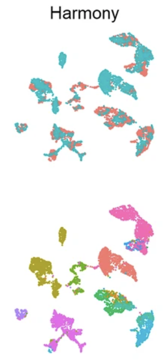
Illustration of what the goal of batch correction is. All these are UMAPs (see Section 3.3.23). The top row colors cells by their batch, and the bottom row colors cells by cell type. (Left) Original data showing batch effects. (Middle) Intermediate processing. (Right) The batch-corrected data. (Tran et al. 2020) ::::
Input/Output. The input to batch correction is (1) either the normalized matrix \(X \in \mathbb{R}^{n\times p}\) or the score matrix \(Z \in \mathbb{R}^{n\times k}\) and (2) an categorical vector \(C \in \{1,\ldots,B\}^n\) which denotes which cell belongs to which batch. (Certain batch correction methods might require more information.) In a literal sense, both \(X\) and \(Z\) are technically row-wise concatenations of many datasets.
If the input is a normalized matrix, the output is a batch-corrected normalized matrix \(X' \in \mathbb{R}^{n\times p}\). If the input is a score matrix \(Z\), the output is a batch-corrected score matrix \(Z' \in \mathbb{R}^{n\times k}\).
Remark (What makes this task statistically possible?). There are many sources of “noise” (i.e., things unrelated to the biology we’re trying to study) in a single-cell dataset.
- Sequencing noise: This comes from the fact that we “randomly” get counts from each cell, and we can’t control how effective each cell is at producing counts. We can think of this as “mean-zero, i.i.d. across all cells” in some sense.
- Batch noise: This is the “noise” that originates from a particular batch. It is probably more statistically appropriate to think of this as a “bias,” because it is not mean-zero. Instead, we conceptually think of this as a shift occurring to all the cells in a batch more-or-less uniformly (but could impact different genes differently).
- Biological confounding noise: Say you want to study how lung tissue changes during aging, but some of your tissue samples come from donors who smoke. The aging biological signature you’re hoping to find would likely be confounded by a smoking signature. This “noise” is also not mean-zero, and it could be different across different cell types. However, given a cell type, this biological confounding effect should be the same across batches. (The trouble is that you might not be aware of all the confounders during an analysis.)
Hence, it is possible to “remove” batch effects because: 1) it’s a constant “shift” for all the cells in the same batch, and 2) we always know the “batches,” since it is purely an artifact of how data is generated. Most batch-correction papers are statistically motivated, but do not have formal theoretical properties. This is primarily due to the fact that in practice, it’s very hard to know how to model a batch effect rigorously. However, there are a few papers that try to leverage this intuition formally in a statistical framework, see (Ma et al. 2024).
Remark (The term “batch” is very overloaded). There are many steps during a single-cell analysis (see Chapter 3). These are some of the things a “batch” could refer to: 1) cells processed together during droplet/gem formation, 2) cells processed during during PCR amplification, 3) cells processed together during sequencing (this is most common usage of the word “batch”), 4) cells processed using different protocols, 5) cells processed by different labs, 6) cells of different donors/organisms, among many more. (The first three steps are similar in “resolution,” but the last three are more “coarse” in how a batch is defined.)
Technically, the statistical logic of most batch-correction methods isn’t suitable for trying to align cells from different donors/organisms since in this setting, the “batches” are based on biology, not a technical artifact. For example, the differences between cells from two donors could be much more complicated than simply cells in two different sequencing batches.
In general, be sure to discuss with the people who generated the data (who likely will have a lot more experience on what technical artifacts are worth worrying about) on how to think about batch effects.
3.3.20 What’s the difference between “batch-correcting” and “adjusting for covariates”?
Technically, there are some batch-correction methods whose premise is to treat each batch as simply a covariate to be adjusted for. The primary example is COMBAT (Zhang, Parmigiani, and Johnson 2020). However, most batch-correction methods do not do this. There is no formal reason why. I personally feel it’s because batch effects is such a critical bottleneck for almost every single-cell analysis that it’s imperative to use a method that is as (sensibly) flexible as possible. See my remark later in Remark 3.2. See (Tran et al. 2020; Luecken et al. 2022) for benchmarking multiple batch correction methods.
3.3.21 A typical choice: Harmony
Harmony (Korsunsky et al. 2019) is one of the most commonly used methods to integrate single-cell datasets from different experiments, technologies, or biological conditions into a shared low-dimensional embedding. The method begins with a principal component analysis (PCA) embedding and iteratively adjusts it to remove batch effects while preserving biological variation. Harmony groups cells into clusters using soft clustering, which assigns cells probabilistically to multiple clusters. These clusters account for technical and biological differences while capturing shared cell types and states. Correction factors are then computed for each cluster and applied to individual cells, ensuring that the final embedding reflects intrinsic cellular phenotypes without being confounded by dataset-specific biases. See Figure 3.17.

3.3.22 How to do this in practice
There is no standardize default for batch correction. The usual practice is to: 1) decide upfront (with your collaborators) on how you would deem what is a “successful” batch correction. This usually involves understanding the data generation protocol and the biology question of interest. This will involve a blend of biological logic (i.e., statements that should be true, given the biological context), qualitative evaluations (i.e., based on plots), and numerical metrics (i.e., based on some score where you decide upfront how the score relates to a desirable batch correction). Then, 2) you try many batch correction methods8.
Remark 3.2. Remark (Personal opinion: Batch correction is single-handedly the most precarious step in almost every analysis). While a cautious statistician might be doubtful for “cherry-picking” a good batch-correction method, the reality is that there is no guaranteed procedure to always work. This is because there are so many types of “batches,” and the underlying data generation pipeline, technology, and biology differs from lab to lab. Also, doing a “bad” batch correction is extremely detrimental. Unlike many other steps in a single-cell analysis where most choices of how to perform a step are “reasonable” (but some methods might have slightly better power or slightly more robust), a bad batch correction can single-handedly invalidate almost all other aspects of a single-cell analysis regardless of how sophisticated those methods are.
Also: batch correction is limited by the experimental design. No “real” way to validate this if you’re only given datasets – the validations need to be decided during the planning of the experimental design. For example, if you are studying cancer, and you put all the cancer donors’ cells in one batch and all the healthy donors’ cells in another batch, then you have no ability to disentangle the batch effects from the biological effect.
To aid validation of batch correction, a common experimental design is to put one reference tissue (where it’s possible to obtain many samples from this one tissue) in every sequencing batch.
3.3.23 Visualization
Visualization is a key step in single-cell sequencing analysis, offering a way to explore and interpret complex datasets intuitively. One of the most popular visualization techniques is Uniform Manifold Approximation and Projection (UMAP), which creates a low-dimensional embedding designed to preserve local and global structure in the data. UMAP is particularly effective for capturing non-linear relationships and revealing clusters of similar cells, making it a powerful tool for visualizing cellular heterogeneity. However, UMAP coordinates are less reliable than those obtained through methods like PCA for quantitative analysis. Unlike PCA, which is grounded in linear transformations and retains a direct link to the original data, UMAP embeddings are highly dependent on parameter choices and random initializations, making them less reproducible. Despite these limitations, UMAP excels as a visualization tool, helping researchers intuitively explore relationships between cells and identify patterns that guide deeper analyses.
Input/Output. The input to visualization is typically the score matrix \(Z\in \mathbb{R}^{n\times k}\) for \(n\) cells and \(k\) latent dimensions, and the output is matrix with \(n\) cells and 2 (sometimes 3) columns, where the visualization is literally plotting the values in the first column against the second column as a scatterplot.
3.3.24 The standard procedure: UMAP
Uniform Manifold Approximation and Projection (UMAP) (Becht et al. 2019) is a dimensionality reduction technique designed to capture both local and global structure in high-dimensional data. UMAP builds on principles of manifold learning, aiming to preserve the topology of the original data in a lower-dimensional space.
- Constructing the high-dimensional graph: UMAP begins by modeling the local neighborhood relationships in the high-dimensional space:
- For each data point \(i\), a probability distribution \(p_{ij}\) is constructed over its neighbors \(j\) based on distances, typically using a kernel function.
- The resulting graph captures the high-dimensional structure of the data.
- Optimizing the low-dimensional embedding: In the low-dimensional space, UMAP aims to construct a graph with similar relationships. It models pairwise probabilities \(q_{ij}\) for the low-dimensional embedding using a smooth, differentiable cost function: \[ C = \sum_{i,j} \left( - p_{ij} \log q_{ij} - (1 - p_{ij}) \log (1 - q_{ij}) \right). \] Here:
- \(p_{ij}\) and \(q_{ij}\) represent probabilities of connectivity in the high- and low-dimensional spaces, respectively.
- The first term encourages similar points in the high-dimensional space to remain close, while the second term discourages unrelated points from being artificially clustered.
- Gradient descent: The low-dimensional coordinates are iteratively optimized using gradient descent to minimize \(C\), aligning the local relationships in the low-dimensional embedding with those in the original space.
UMAP excels at preserving local neighborhoods while maintaining some global structure, making it particularly effective for visualizing high-dimensional single-cell RNA-seq data. However, the resulting embeddings depend on hyperparameters (e.g., number of neighbors, minimum distance) and are not designed for quantitative analysis, as they do not preserve metric properties of the original data. See https://github.com/jlmelville/uwot for great in-depth discussions on UMAPs.
Remark (Yes, UMAPs are also a “dimension reduction,” but they serve a very different purpose). You can think of UMAPs as a very specific dimension reduction where \(k\) is always 2 or 3. However, UMAPs serve a very different role – very few single-cell analyses relies on the UMAP coordinates, but many single-cell methods rely upon the low-dimensional vector \(Z_{i,\cdot}\in\mathbb{R}^k\) from a dimension reduction method.
The reason is that UMAPs are usually solely for visualizations and nothing else. There is almost no concrete relation between the distance between any two cells based on their UMAP coordinates and their true dissimilarity based on their gene expression profiles. The most common analogy is to think of visualizing the Earth on a 2D map, see Figure 3.18. No matter how you try to draw the world on a sheet of paper, there’s always some unnatural distortion. If you interpret this map very literally, it seems like California is further away from Japan than Spain is, and Antartica is almost as large as all the other continents combined. The point is, every low-dimensional projection always sacrifices some aspects, and when you try projecting high-dimensional data to specifically only 2 dimensions, a lot of large-scale qualities “break.”
See (Prater and Lin 2024) for more discussions about how to think about UMAPs, Figure 3.19. There’s a big debate on what is “acceptable” or “not acceptable” to infer from UMAPS. See (Chari and Pachter 2023; Lause, Berens, and Kobak 2024), and a recent large controversy in genetics (https://www.science.org/content/article/huge-genome-study-confronted-concerns-over-race-analysis).
My take: UMAPs are a useful visualization tool (in the sense that it’ll be ridiculous to claim we should never visualize our data, and we should just accept every visualization tool will have its own drawbacks). However, you should have quantitative metrics planned out prior to visualization so you’re not solely relying on UMAPs for your analysis. UMAPs are useful for giving you a sense of the data quality and broad cellular relations before investing time to carefully quantify the biology of interest. Your biological evidence should not solely rely on UMAPs.


3.3.25 Relation to PCA
UMAPs are most related to the Formulation #3 of PCA Equation 3.6. Specifically, instead of “\(D_X\)” and “\(D_{XW}\)” (originally measuring the distance between two cells using Euclidean distance), UMAPs instead use an adaptive kernel on a cell-cell graph to measure the similarity between two cells, and the loss function isn’t simply a difference between the two similarities.
3.3.26 How to do this in practice
See the Seurat::RunUMAP function, illustrated in Figure 3.20. The resulting visualization is shown in Figure 3.21.


Seurat::DimPlot(pbmc, reduction = "umap") function to visualize the first two PCs. See the tutorial in https://satijalab.org/seurat/articles/pbmc3k_tutorial.html.
3.3.27 A brief note on other approaches
Because visualizing high-dimensional data will always be a need, and there’s never going to be an “optimal” way to do it, the visualization method of choice is going to change based on the community’s desires every 5-10 years. While currently UMAP is king (which dethroned t-SNE, who was the previous king), there’s definitely methods trying to dethrone UMAP. The method I’ve seen the most popularity to dethrone UMAP so far is PaCMAP, but as of 2024-25, UMAP is still by far the most common visualization method. See (Huang et al. 2022) for a broad benchmarking of such methods.
There are two lines of work I’ll mention that might be of interest for the statistical students. One is developing methods to assess how “distorted” the visualization is, see (Johnson, Kath, and Mani 2022; Xia, Lee, and Li 2024). Another is to trying to prove (using a formal statistical model) how well these visualization methods actually “cluster” the cells, see (Arora, Hu, and Kothari 2018; Cai and Ma 2022).
You can have a simple hierarchical model in your head – each human donor contributes one (or more) tissue sample. Each tissue sample contains many cells.↩︎
How many genes are there in the human body? This is not a well-defined questions. If you want to only ask about protein-coding genes, there’s probably about 24,000 of them (Salzberg 2018). However, most gene callers (such as CellRanger https://www.10xgenomics.com/support/software/cell-ranger/latest, which is what we usually use for 10x single-cell data) also label genes that don’t translate. We’ll talk about this in Section 4.8.↩︎
Typically, the feature selection step doesn’t use the normalized matrix even though normalization happens before feature selection. See https://github.com/satijalab/seurat/blob/ece572a/R/preprocessing.R#L3995. This is because it’s preferable to normalize using all the reads, even from genes you don’t actually include in your analysis.↩︎
Typically, the feature selection step doesn’t use the normalized matrix even though normalization happens before feature selection. See https://github.com/satijalab/seurat/blob/ece572a/R/preprocessing.R#L3995. This is because it’s preferable to normalize using all the reads, even from genes you don’t actually include in your analysis.↩︎
Sometimes, people use the word “overcrowding” to refer to the fact that embedding methods might collapse nearby points too aggressively.↩︎
See Seurat’s recommendation in https://satijalab.org/seurat/articles/seurat5_integration.↩︎