7 ‘Single-cell’ DNA
7.1 Genetics 101
Understanding the fundamental concepts of genetics is essential for studying genomic variation, including copy-number variations (CNVs) and single nucleotide polymorphisms (SNPs). This section provides an overview of genetic architecture, SNPs and their detection, commonly sequenced tissues, and genome annotation resources such as the UCSC Genome Browser.
Single Nucleotide Polymorphisms (SNPs) and Their Detection.
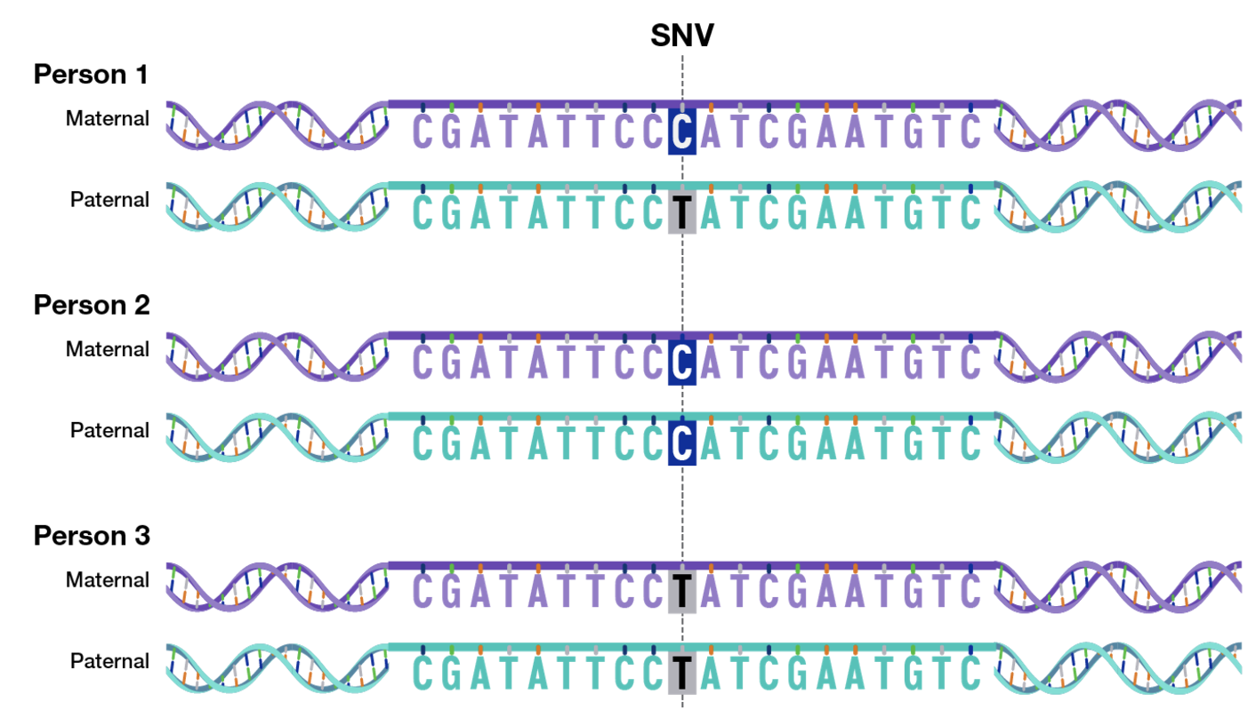
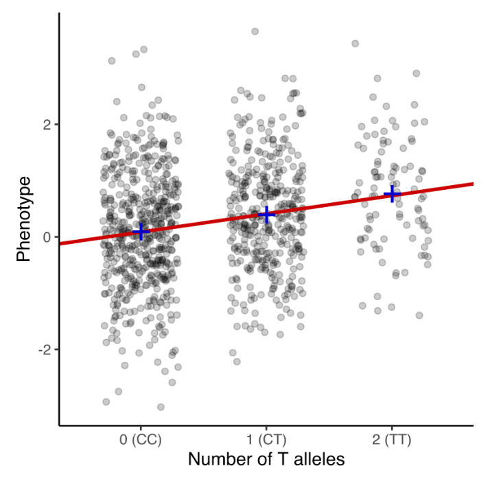
A single nucleotide polymorphism (SNP) is a variation at a single base pair position in the genome that is present in a significant fraction of the population. SNPs are the most common type of genetic variation and can have functional consequences depending on their location. When an SNP occurs within a coding region, it may alter the resulting protein sequence if it leads to an amino acid substitution (nonsynonymous SNP) or have no effect if the change is synonymous. SNPs in noncoding regions can impact gene regulation by affecting transcription factor binding sites, splicing efficiency, or untranslated regions (UTRs). Since you have “two copies” of each of your 23 chromosomes, this means SNP data is a data matrix of \(n\) people by \(p\) SNP regions (think of a couple million – more on this technicality later), where each value is \(\{0,1,2\}\), see Figure 7.1. Typically, the major allele is defined as “0”, and a “1” or “2” means if how many copies of the minor allele do you have.
SNPs are detected using high-throughput sequencing technologies, primarily whole-genome sequencing (WGS) and whole-exome sequencing (WES). In these approaches, DNA is extracted from a biological sample, fragmented, and sequenced to generate short or long reads. The raw sequencing reads are then aligned to a reference genome, and variant calling algorithms such as those implemented in GATK (McKenna et al. 2010), bcftools, and FreeBayes (Garrison and Marth 2012) identify SNPs by comparing observed nucleotide differences to the reference sequence. (See Zverinova and Guryev (2022) for a overview). The sequencing depth, or coverage, at a given genomic position determines the confidence in an SNP call, with higher coverage reducing the likelihood of sequencing errors.
7.1.0.1 Tissues Used for DNA Sequencing
The choice of tissue for sequencing depends on the research objective. In population genetics and germline variant studies, DNA is typically extracted from peripheral blood or saliva, as these sources provide a reliable representation of an individual’s inherited genome. For cancer studies and somatic mutation analysis, tumor biopsies and matched normal tissue (such as blood or adjacent non-tumor tissue) are commonly sequenced to distinguish acquired mutations from germline variants. Additionally, single-cell sequencing has enabled the study of genetic heterogeneity within complex tissues, allowing researchers to profile CNVs and SNPs in individual cells from a given sample.
7.1.0.2 Gene Architecture and Functional Elements
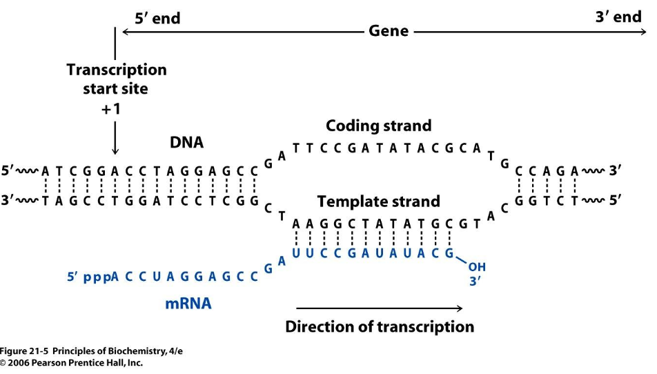
The structure of a gene consists of multiple regions that contribute to its regulation, transcription, and translation. A gene typically includes a promoter region, which contains binding sites for transcription factors and RNA polymerase, playing a crucial role in gene expression regulation. The transcription start site (TSS) marks the beginning of RNA synthesis. The gene body consists of exons, which encode protein sequences, and introns, which are transcribed but spliced out during mRNA processing. The untranslated regions (UTRs), found at the 5’ and 3’ ends of the mature mRNA, influence mRNA stability, localization, and translation efficiency. Alternative polyadenylation (APA) sites within the 3’ UTR can affect transcript stability and cellular localization, providing an additional layer of post-transcriptional regulation.
Splicing is a critical process that removes introns from pre-mRNA and joins exons to form a mature transcript. Alternative splicing allows a single gene to produce multiple transcript isoforms, greatly expanding the diversity of the proteome. Mutations or polymorphisms in splicing regulatory elements can disrupt normal splicing patterns, leading to disease-associated transcript variants.
7.1.0.3 Protein-Coding and Noncoding Regions of the Genome
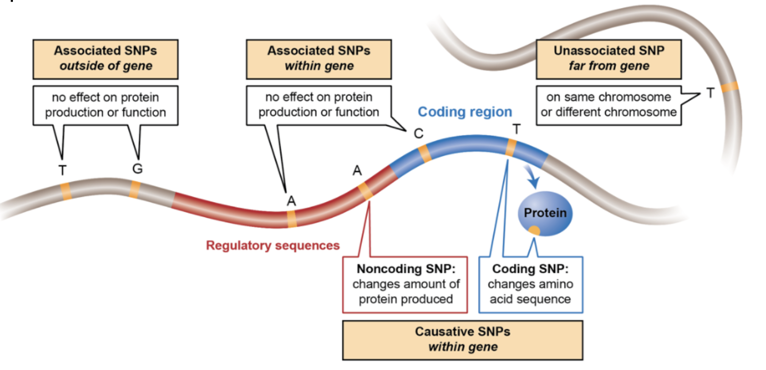
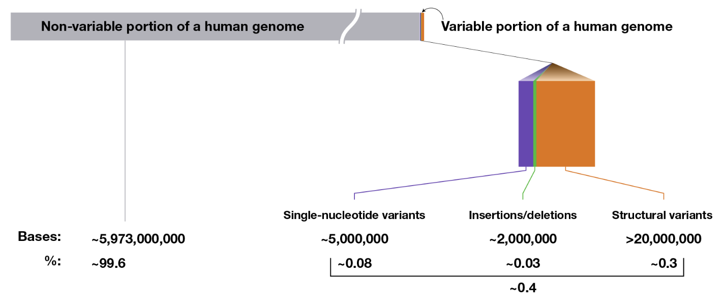
The human genome consists of approximately 3 billion base pairs, yet only a small fraction of this sequence directly encodes proteins. Protein-coding genes occupy approximately 1–2% of the genome, corresponding to around 20,000 protein-coding genes. However, these genes are distributed across the genome, with some regions containing high gene density while others are gene-poor. Despite the low proportion of protein-coding DNA, the noncoding genome plays an essential role in gene regulation, chromatin organization, and cellular function. Noncoding regions include promoters, enhancers, silencers, insulators, and noncoding RNAs (such as microRNAs and long noncoding RNAs) that modulate gene expression. SNPs can lie in any of the regions, see Figure 7.2.
7.1.0.4 Exploring Genomic Annotations: The UCSC Genome Browser.
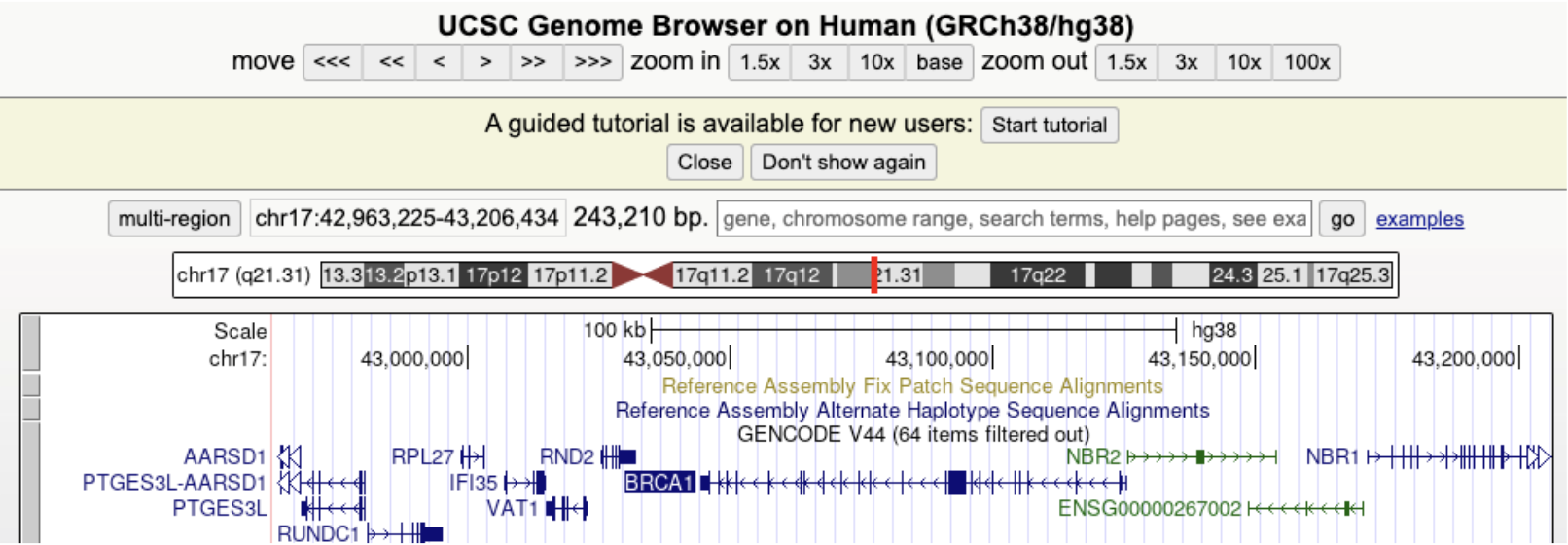
The UCSC Genome Browser is a widely used web-based platform that provides interactive visualization of genomic annotations, including gene structures, SNP locations, and regulatory elements. Researchers use the UCSC Genome Browser to explore gene architecture, examine conservation across species, and analyze experimental data such as RNA-seq and ChIP-seq tracks. The browser integrates multiple annotation tracks that display exon-intron boundaries, transcription factor binding sites, chromatin accessibility, and population-level variant frequencies. By selecting relevant tracks, users can assess how SNPs or CNVs may influence gene function and expression.
See Figure 7.3, Figure 7.4, and Figure 7.5 for an example of how to use the UCSC browser.
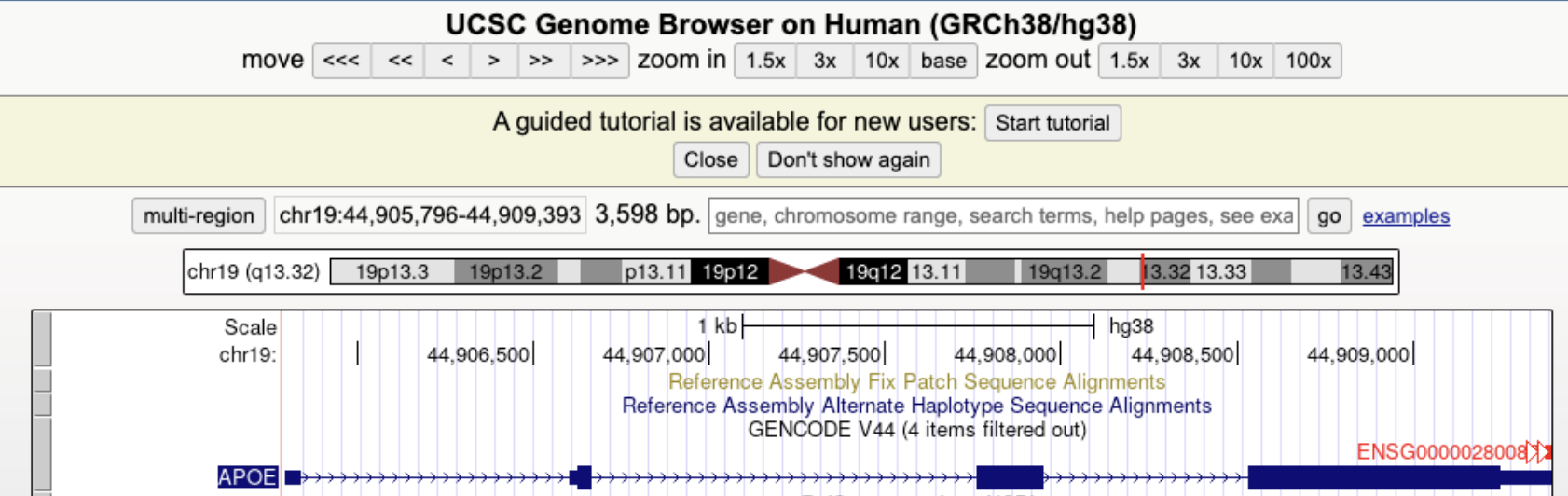
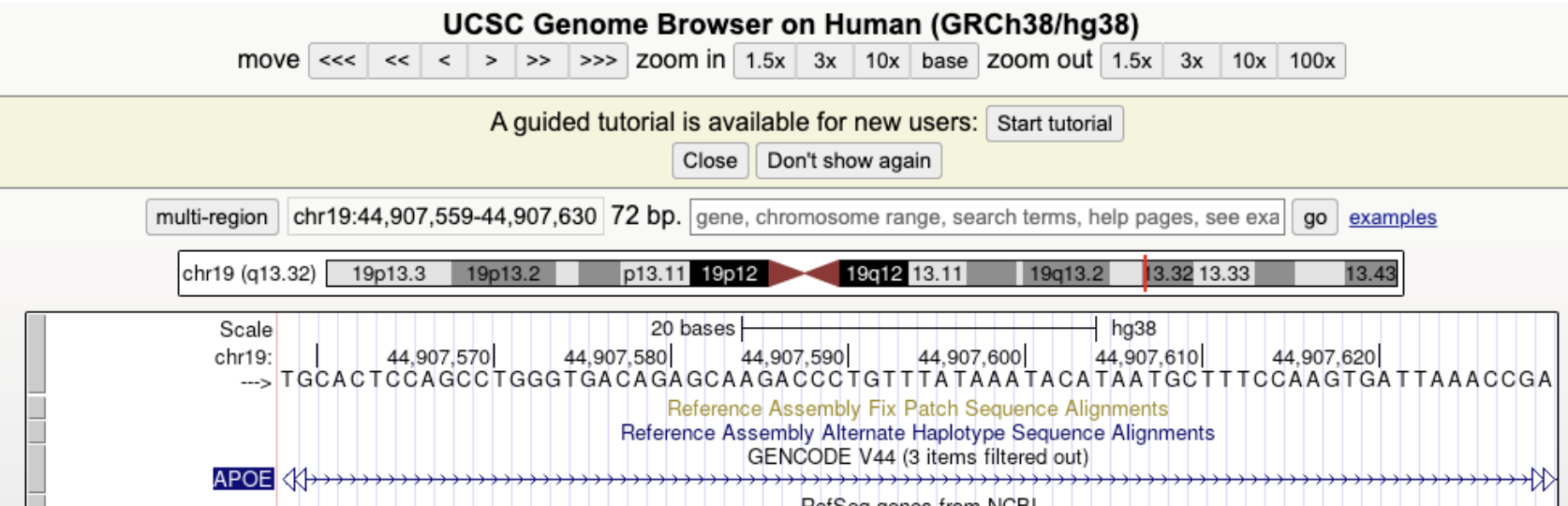
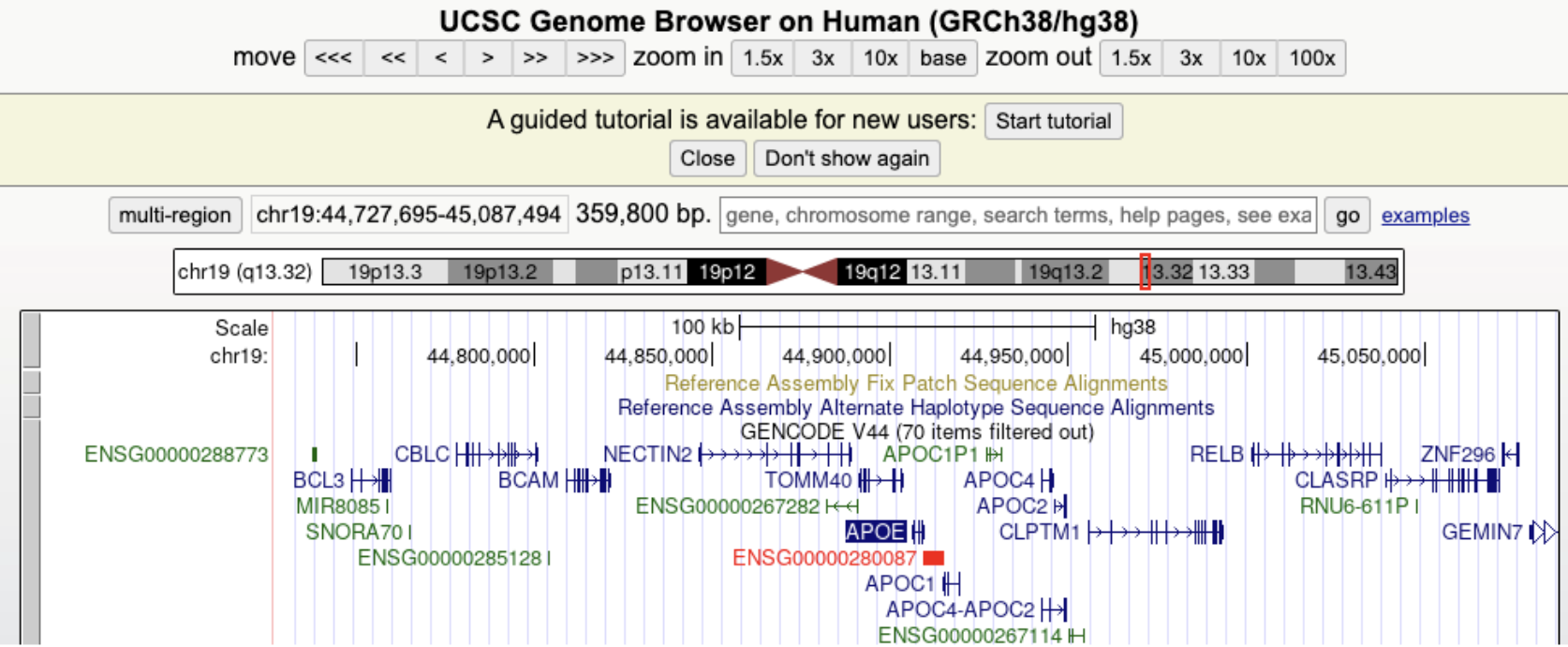
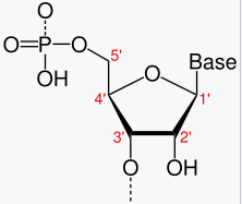
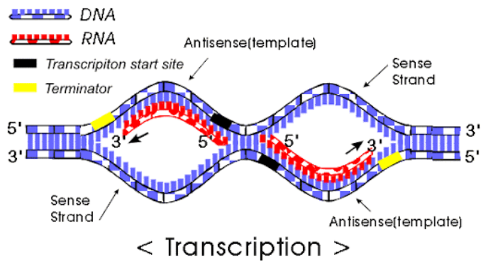
Figure 7.6 demonstrates that you can tell which side of the chromsome the DNA is on. Why are there sides? Remember that transcription always goes from the 5’ end to 3’ end1, see Figure 7.7, Figure 7.8, Figure 7.9. mRNA is single-stranded, so you need to know which strand the DNA template is from.
7.2 A brief blurb about GWAS
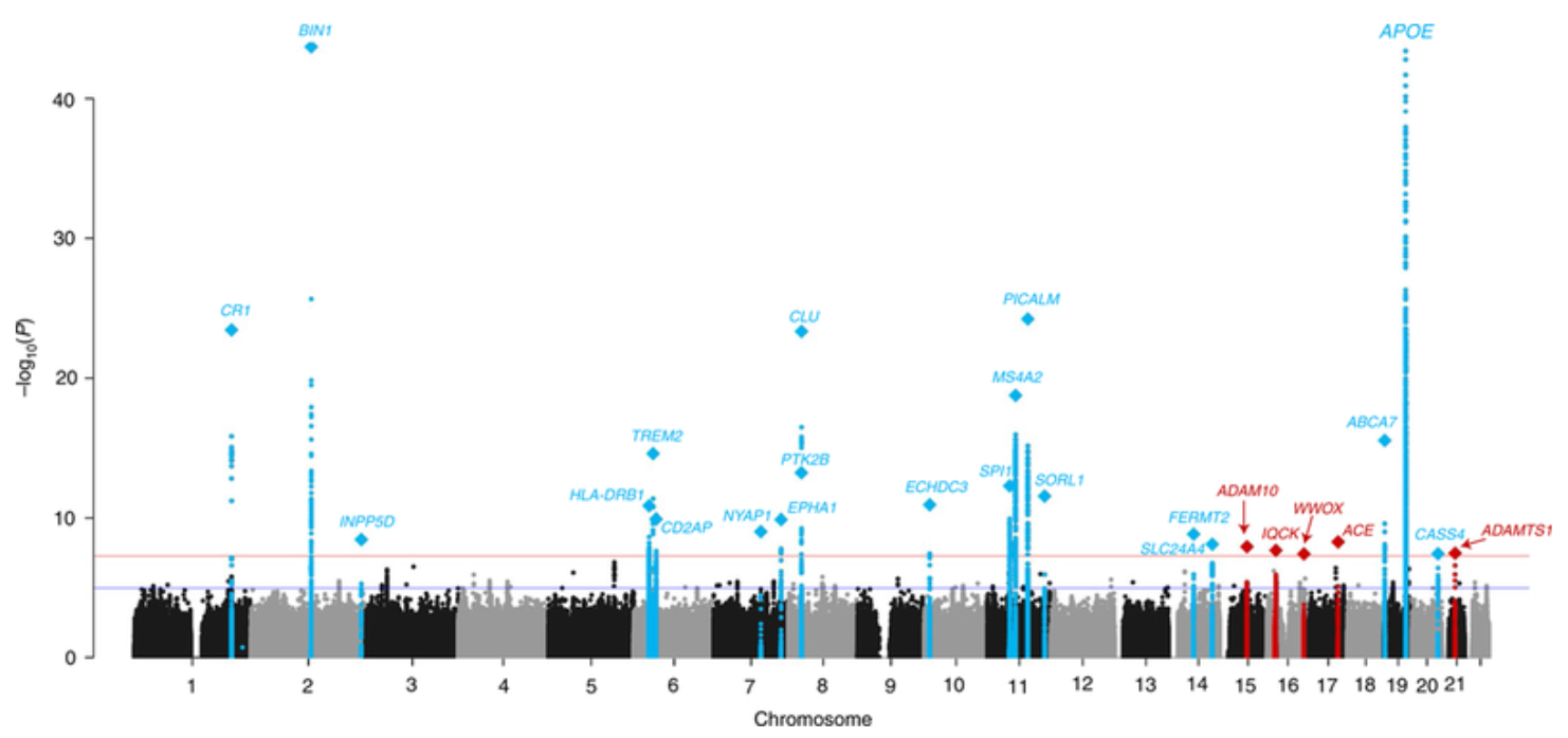
Genome-wide association studies (GWAS) analyze genetic variation across a population to identify single nucleotide polymorphisms (SNPs) associated with a phenotype of interest. The data consist of \(n\) donors, each genotyped at \(p\) SNPs, where \(p\) typically ranges from hundreds of thousands to millions. To enhance statistical power, imputation is commonly performed to infer unobserved genotypes based on reference panels, effectively increasing the number of analyzed SNPs. The association of each SNP with the phenotype is tested using regression models, often accounting for population stratification and relatedness through principal components or mixed models, see Figure 7.10. The results are visualized in a Manhattan plot, where each SNP’s \(-\log_{10}(p)\) value is plotted against its genomic position, highlighting loci with strong associations as peaks above the genome-wide significance threshold, see Figure 7.11. See https://i2pc.es/coss/Docencia/statisticalHelper/GWAS.pdf for the basics of a GWAS analysis.
7.2.0.1 Fine mapping and other methods to get more “causal” variants.
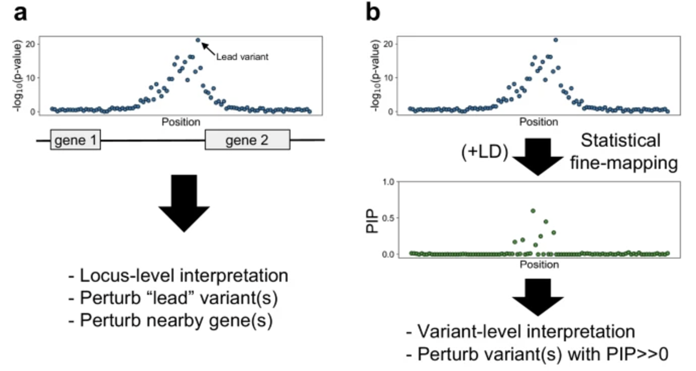
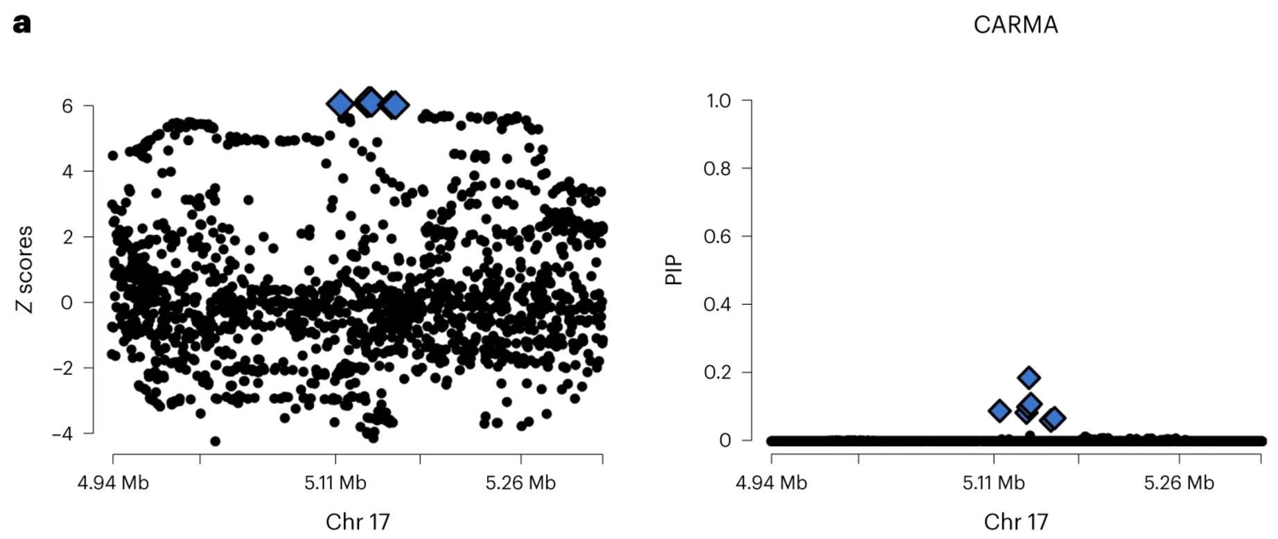
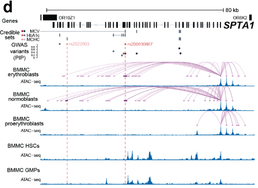
Due to linkage disequilibrium (LD) and other factors, genetic variants are often highly correlated across a chromosome, leading to clusters of significant SNPs in GWAS results. Fine-mapping aims to disentangle these associations by leveraging LD patterns to identify the variants most likely to be causal. This is typically done using Bayesian or probabilistic approaches that assign posterior inclusion probabilities (PIPs) to SNPs, quantifying their likelihood of being causal, as illustrated in Figure 7.12. Methods such as CAVIAR Hormozdiari et al. (2014), SuSiE G. Wang et al. (2020), and FINEMAP Benner et al. (2016) integrate GWAS summary statistics with LD information to refine candidate variants. For some alternatives that are more causal in statistical flavor, see GhostKnockoff He et al. (2022). The impact of fine-mapping can be seen in Figure 7.13, where prioritization of variants reduces uncertainty and improves biological interpretability.
7.2.0.2 Some videos to look at for fun.
- “How They Caught The Golden State Killer” (Veritasium): https://www.youtube.com/watch?v=KT18KJouHWg
7.2.1 Before we get too far, a quick note about the types of genetic variations
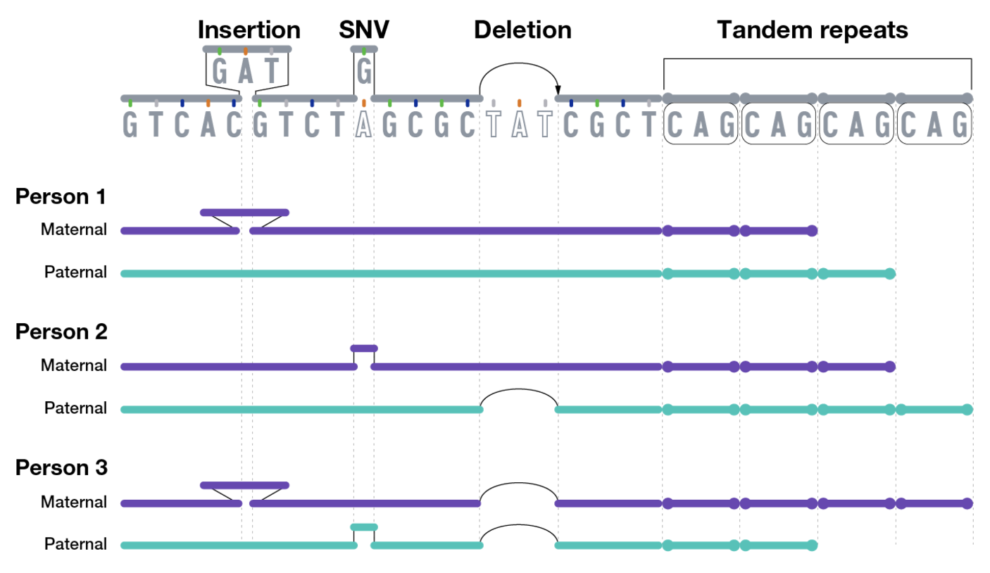
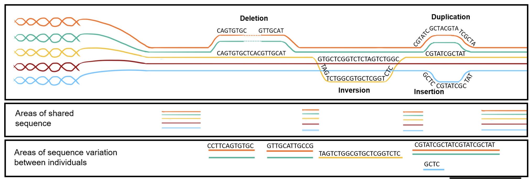
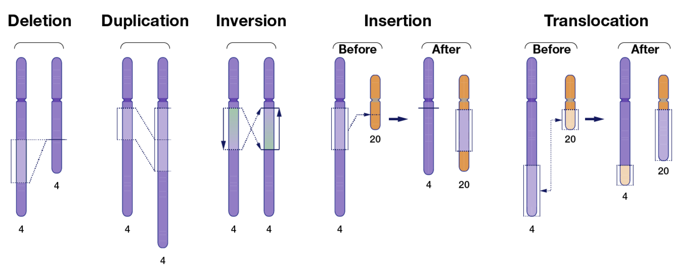
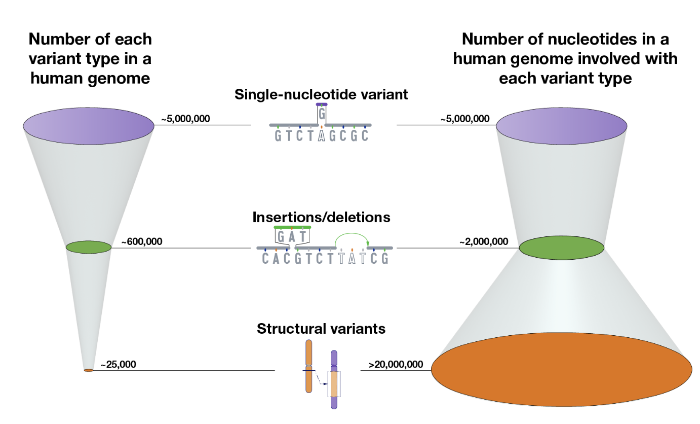
Genetic variation arises from different types of mutations and structural alterations in the genome. See Figure 7.14 and Figure 7.16.
- Single Nucleotide Variant (SNV): A single base change in the DNA sequence, which can be synonymous, missense, or nonsense depending on its impact on protein coding.
- Insertions and Deletions (Indels): The addition or removal of a small segment of DNA, which can cause frameshift mutations if they occur in coding regions.
- Inversions: A segment of DNA is reversed within the chromosome, potentially disrupting gene function or regulation.
- Tandem Repeats: Short DNA sequences repeated in succession, which can expand in diseases like Huntington’s. You’re usually think of a very short sequence (10 base pairs or less) that are repeating very often.
- Copy Number Variations (CNVs): Large duplications or deletions of genomic regions, affecting gene dosage and expression. You’re usually thinking of a very long segment of the chromosome, ranging to 1000 to millions of base pairs that are repeated.
- Translocations: The exchange of genetic material between non-homologous chromosomes, which can lead to fusion genes and genomic instability.
7.2.2 A brief note about the IGV
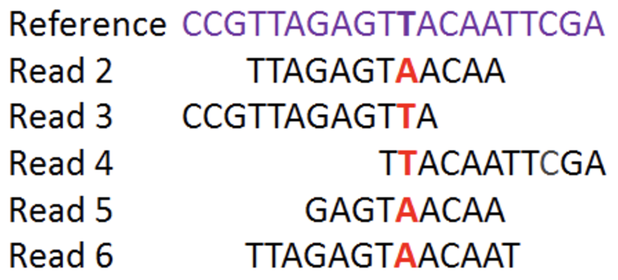
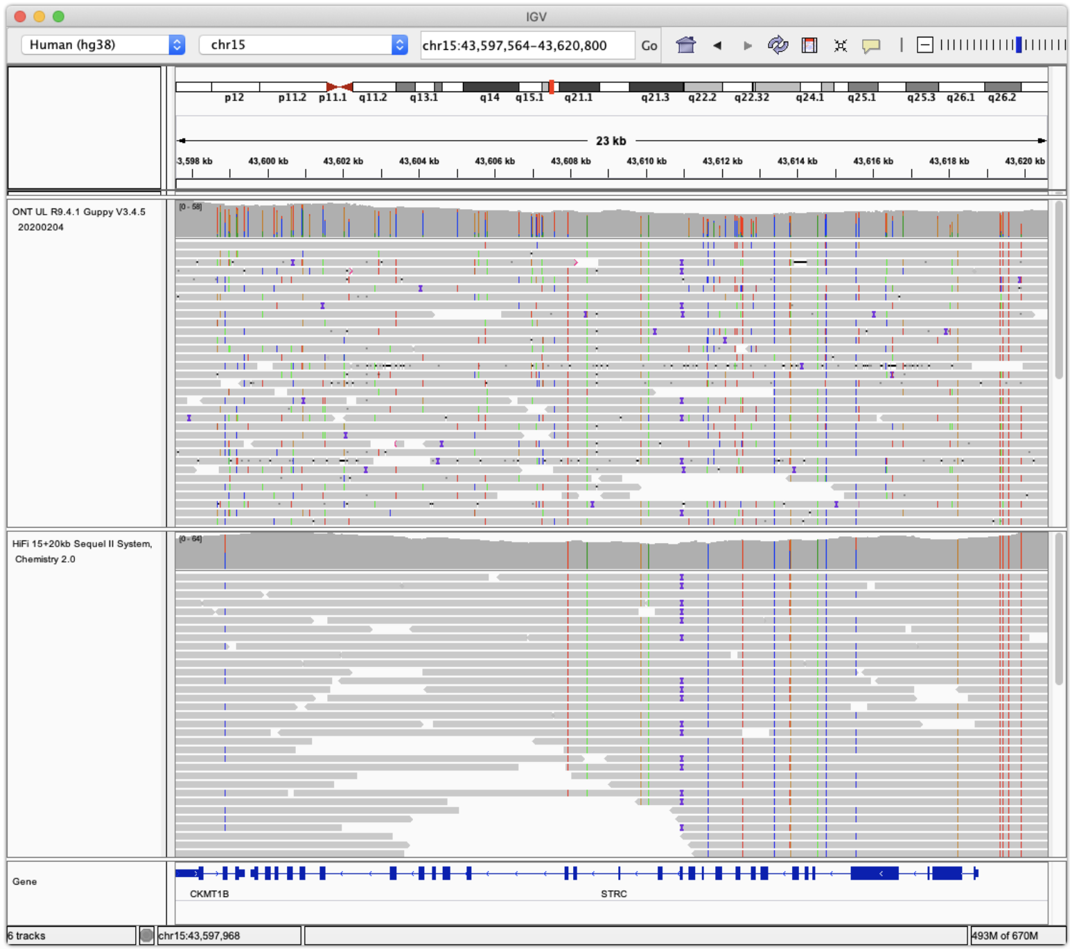
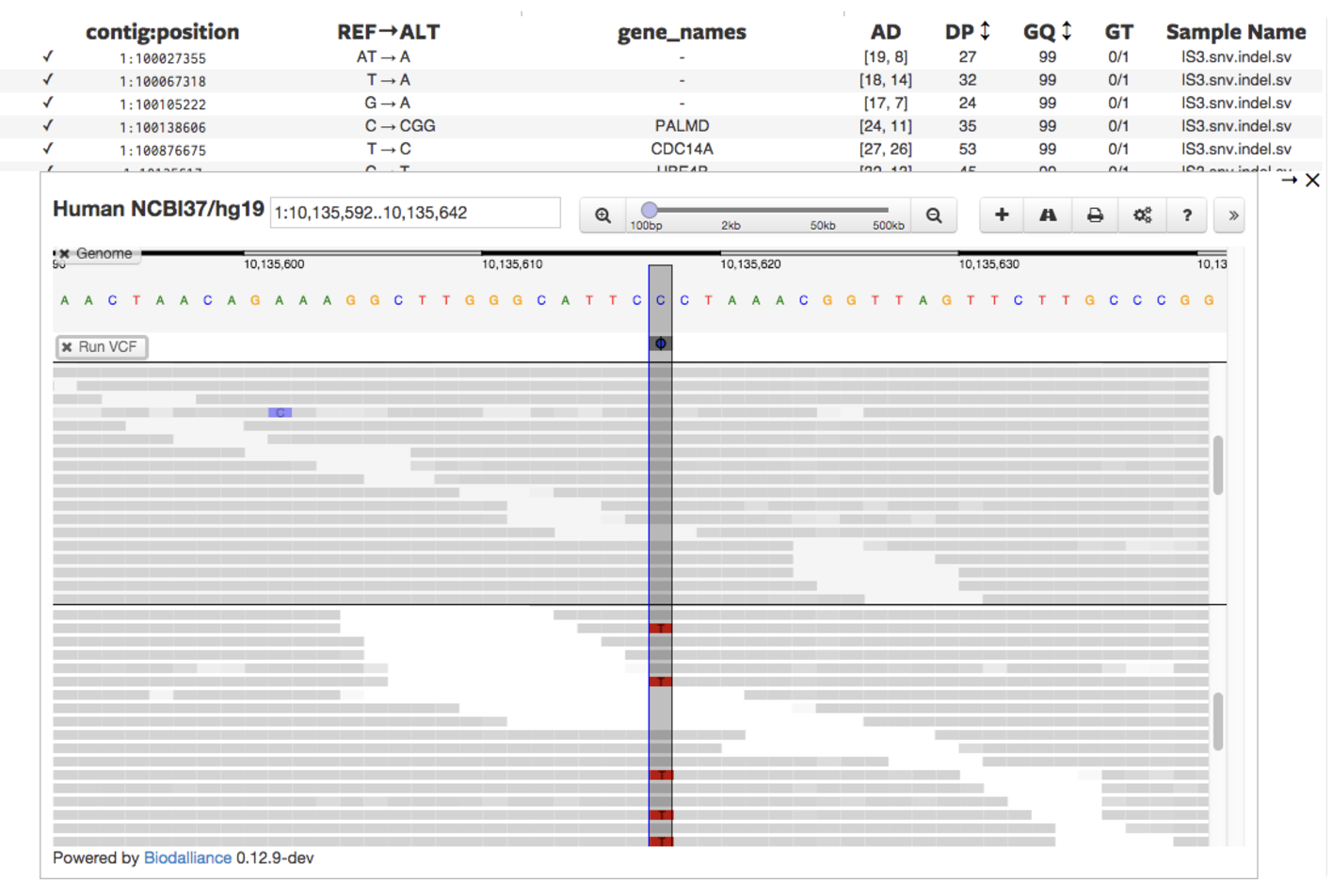
The Integrative Genomics Viewer (IGV) is a powerful tool for visualizing raw sequencing reads in a genomic context through pileup plots. See Figure 7.19 for what a “pileup” is. IGV allows users to examine aligned reads against a reference genome, displaying key features such as exons and introns of annotated genes, as well as the reference sequence itself. Individual sequencing reads are shown with base-level resolution, highlighting mismatches to the reference, including SNPs, small insertions and deletions, and structural variations such as inversions. IGV also marks sequencing errors with quality scores, enabling users to assess confidence in variant calls. By interactively navigating across genomic regions, zooming in on loci of interest, and customizing track displays, IGV facilitates the interpretation of raw sequencing data with high precision. See Figure 7.20 and Figure 7.21 as an example.
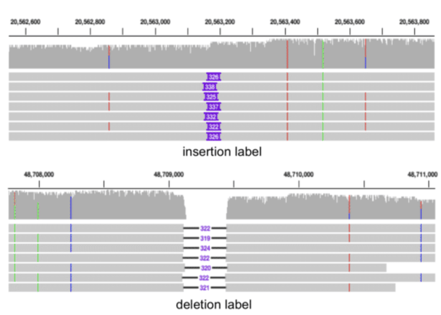
The IGV (depending on the version and settings) can also show insertions and deletions (see Figure 7.22), as well as inversions.
7.2.3 If you thought scRNA-seq data was complicated…
While single-cell RNA-seq presents significant analytical challenges, studying genetics—particularly large-scale genome-wide association studies (GWAS) and population genetics—introduces an entirely new set of complexities:
Linkage disequilibrium and evolutionary constraints:
Unlike scRNA-seq, where gene expression is not typically inherited (and hence, why we can still do incredible genomic analyses with samples from very few people), genetic variants are often inherited together due to linkage disequilibrium (LD). This means that interpreting the effect of a single variant requires understanding its entire haplotype structure. Additionally, selective pressures shape the distribution of variants across populations, making genetic associations highly context-dependent.Structural variation beyond SNPs:
scRNA-seq primarily deals with gene expression counts, but genetic variation extends beyond single nucleotide polymorphisms (SNPs). Structural variations, such as short tandem repeats (STRs) and copy number variations (CNVs), can have significant functional consequences yet are much harder to detect and analyze (see Chapter 6).Reference genome challenges:
While single-cell studies align reads to a standard reference genome, genetic studies must carefully consider population-specific variation and potential biases in reference genomes. Reference panels are crucial for variant calling, yet no reference is truly comprehensive, leading to systematic errors in certain populations. See Chapter 6.Necessity of imputation:
Unlike transcriptomics, where missing values are typically ignored, genetic studies require imputation to infer unobserved variants, ensuring more comprehensive variant coverage. Genotyping arrays typically measure around 500,000 to 1,000,000 SNPs directly, but many common genetic variants remain untyped. Imputation leverages linkage disequilibrium (LD) patterns and large reference panels, such as 1000 Genomes or UK Biobank, to predict genotypes at millions of additional loci. After imputation, the number of SNPs analyzed can increase to 10–50 million, greatly enhancing the resolution of downstream association studies. Tools such as the Michigan Imputation Server and Beagle facilitate this process, albeit with a significant increase in computational complexity.Massive dataset sizes and privacy constraints:
Single-cell datasets typically contain tens to hundreds of thousands of cells, but genetic datasets can involve millions of individuals (e.g., UK BioBank). This introduces logistical challenges in data storage, processing, and access control, as genetic data must be handled under strict privacy regulations.
For this reason, many methods that analyze genetics (DNA) have to be designed to accommodate using the summary statistics of a study. As one example (among many), see Zou et al. (2022), which extends SuSIE G. Wang et al. (2020) to handle only summary statistics.
Typically, these methods using summary statistics are “meta-analyses,” which combine many cohorts (which contain different people from different populations) to (hopefully) increase the overall statistical power.Increased bioinformatics and computation demands:
scRNA-seq pipelines rely on well-established tools for alignment, quantification, and clustering, but genetic studies demand a broader and more complex bioinformatics workflow, including variant calling, quality control, imputation, GWAS modeling, and fine-mapping. Analyzing genetic data often requires specialized HPC environments due to the scale of computations.
7.3 … As an aside: Does my DNA mutate over my life?
Somatic mutations – those arising in non-germline cells – accumulate throughout an individual’s lifetime and are key contributors to genetic mosaicism. Studies indicate that somatic mutations can occur at every stage of development and continue to arise during adulthood, driven by normal cell division, environmental insults, and other factors.
Importantly, research has shown that even healthy tissues, such as blood or brain, may harbor these post-zygotic changes that were not inherited from parental genomes.
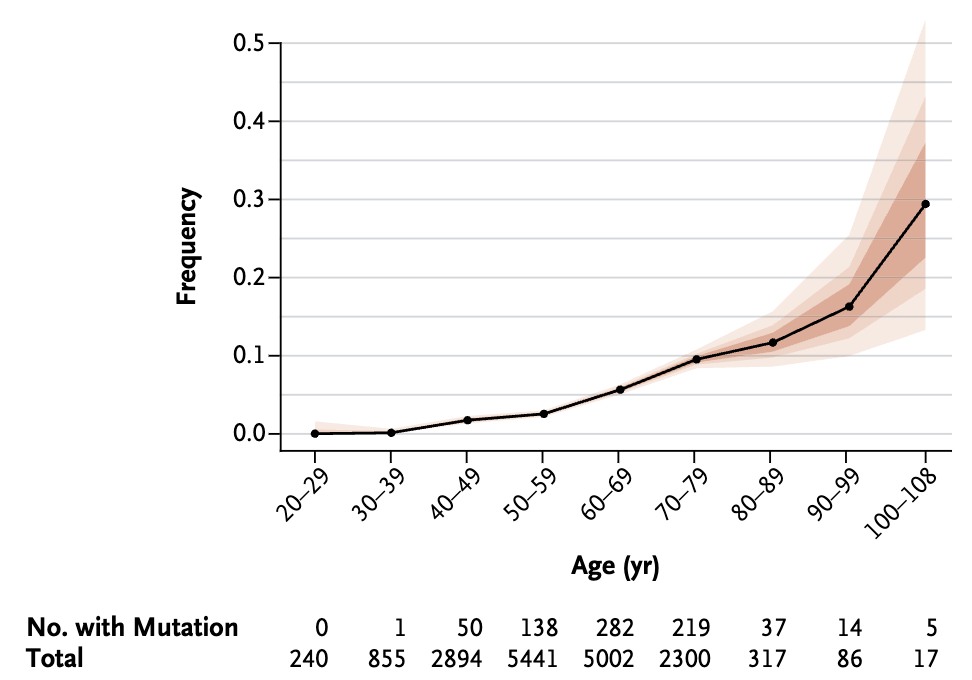
The frequency of somatic mutations tends to increase with age, as documented in hematopoietic cells and other tissues where clonal expansions of mutated cells have been observed Figure 7.23.
In some individuals, the accumulation of such changes remains relatively modest, whereas in others, especially at older ages, hypermutability or clonal dominance may emerge, potentially affecting organ function or predisposing to disease, see more details in Bae et al. (2022). These findings highlight that our DNA, far from being static, undergoes changes over time that can have significant biological consequences. See Milholland et al. (2017) for studies of the mutation rate.
The importance of studying somatic mutations lies in understanding both normal physiology and disease pathogenesis.
While many somatic variants are functionally silent, others can affect cell growth, alter gene expression in critical pathways, or provide selective advantages to clones. Tracking these mutations illuminates how tissues develop, age, and sometimes transition to pre-malignant or malignant states.
Moreover, the detection of specific mutation profiles in otherwise healthy tissue can serve as an early biomarker for conditions such as cancer and neurodegenerative disorders, and may also provide insights into the process of brain development and function, see potential evidence in Bouzid et al. (2023).
Thus, clarifying how frequently somatic mutations arise and determining how these mutations shape cellular behavior form a vital cornerstone for medical research and potential future therapies.
7.4 Studying Single-Cell eQTL
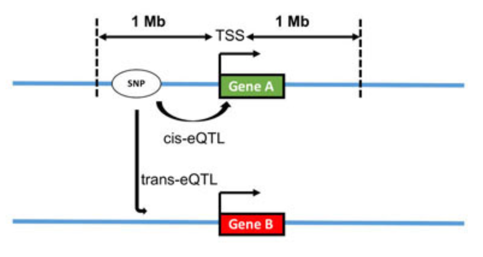
Expression Quantitative Trait Loci (eQTL) analysis is a fundamental approach for linking genetic variation to gene expression levels, offering insights into how genetic differences influence transcriptomic regulation, see Figure 7.24. Traditional eQTL studies rely on bulk RNA sequencing data, which averages gene expression across many cells within a tissue. However, with the advent of single-cell RNA sequencing (scRNA-seq), researchers can now perform single-cell eQTL (sc-eQTL) analyses, enabling the detection of genetic effects on gene expression at a much finer resolution.
One of the key advantages of sc-eQTL analysis is its ability to account for cellular heterogeneity, a limitation in bulk RNA-seq studies. Different cell types within a tissue can have distinct gene regulatory mechanisms, and bulk eQTL studies may obscure these effects by averaging signals across cell populations. Single-cell approaches, in contrast, allow researchers to stratify eQTL analysis by cell type, uncovering cell-type-specific regulatory interactions that may be masked in bulk data. Additionally, sc-eQTL studies enable the exploration of dynamic regulatory effects in response to stimuli, capturing transient gene expression changes driven by genetic variants (see Figure 4 of Yazar et al. (2022)).
Beyond identifying associations between SNPs and gene expression, eQTL analysis can provide insights into enhancer regulation by determining whether an enhancer region containing a SNP is linked to gene expression changes at a target gene, see Figure 7.25. This is particularly useful for understanding non-coding regulatory elements that may influence disease risk.
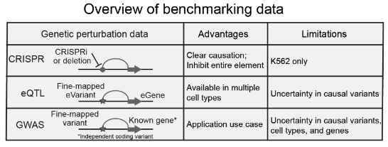
Compared to genome-wide association studies (GWAS), which identify statistical associations between SNPs and phenotypic traits without necessarily indicating causality, eQTL studies provide functional insights into how genetic variation affects transcriptional regulation. However, eQTL analyses alone cannot establish direct causal relationships, unlike CRISPR-based perturbation approaches such as knockouts or CRISPR interference (CRISPRi), which can experimentally validate whether a SNP within a regulatory region directly modulates gene expression. See Figure 7.26.
The process of conducting sc-eQTL analysis involves several computational steps. First, scRNA-seq data is preprocessed to correct for technical noise and batch effects, often using normalization methods tailored for sparse single-cell data. Next, genetic variants are genotyped using whole-genome sequencing (WGS) or genotype imputation from single-nucleotide polymorphism (SNP) arrays. Gene expression values and genetic variants are then correlated to identify eQTLs, typically using linear mixed models or Bayesian approaches that account for population structure and technical confounders. Because single-cell datasets are noisier and lower in coverage compared to bulk sequencing, careful modeling of dropout effects and overdispersion in expression data is essential.
7.4.0.1 Performing your own eQTL.
At a high level, methods to perform GWAS (or fine-mapping, or other follow-up downstream analyses to hone in on more likely causal variants, mentioned in [Section @ref(sec-gwas)]) are sometimes repurposed for an eQTL analyses. Typically, you have genetic information of each donor and then scRNA-seq from these same donors. Then, you process the scRNA-seq data to focus on one particular cell-type in your eQTL analysis. To do this, you take all the gene expression (across many donors, but for just one cell type) to from pseudo-bulk gene expressions (one expression profile per donor), and then perform the following regression. See https://rpubs.com/MajstorMaestro/349118 or papers like T. Wang et al. (2021) to see how to perform an eQTL analyses. (These are not for single-cell variations.)
Here are some additional details. The following procedure is used in many papers, such as Yazar et al. (2022). To perform sc-eQTL mapping for a specific cell type, expression levels are aggregated using a pseudobulk approach, and associations between genotype and expression are tested while controlling for confounding factors.
Consider a cohort of \(n\) individuals, each providing scRNA-seq data. Let \(G_i\) represent the genotype at a given SNP for individual \(i\), encoded as the minor allele count (0, 1, or 2 under an additive model). Let \(Y_i^{\text{bulk}}\) denote the pseudobulk expression level of a gene of interest for individual \(i\), obtained by summing or averaging expression across cells of the target type. We model the pseudobulk expression as: \[ Y_i^{\text{bulk}} = \beta_0 + \beta_1 G_i + \gamma^\top C_i + u_i + \epsilon_i, \] where \(\beta_1\) quantifies the eQTL effect, \(C_i\) represents individual-level covariates such as age, sex, genetic ancestry principal components (PCs), and batch effects, \(u_i\) is a random effect capturing inter-individual variation, and \(\epsilon_i\) is the residual error. (Here, you’re thinking of \(Y_i\) as a gene, and \(G_i\) is any SNP that is close to the gene, and we’ll elect a particular SNP as the eQTL hit (until we do a follow-up fine-mapping analysis) based on which one is the most significant.) To reduce technical and biological confounding, we incorporate Probabilistic Estimation of Expression Residuals (PEER) factors Stegle et al. (2010), which model hidden confounders affecting gene expression. PEER decomposes expression variation into structured components, allowing removal of unwanted effects such as batch effects, library size, and latent population structure.
Beyond standard eQTL detection, we perform conditional cis-eQTL analysis to identify secondary genetic variants affecting expression after accounting for the top associated SNP. Given an initially detected cis-eQTL variant \(G_i^{(1)}\), we extend the model: \[ Y_i^{\text{bulk}} = \beta_0 + \beta_1 G_i^{(1)} + \beta_2 G_i^{(2)} + \gamma^\top C_i + u_i + \epsilon_i, \] where \(G_i^{(2)}\) is an additional SNP in the cis-regulatory region of the gene. This analysis helps identify independent regulatory variants within the same locus.
7.4.0.2 What are on earth are these “genetic ancestry” and “unmeasured confounders”?
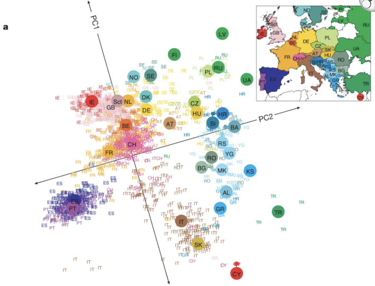
Genetic ancestry and unmeasured confounders are critical considerations in eQTL and GWAS study design. Most genetic studies are conducted in cohorts with limited ethnic diversity to reduce population structure effects, but even within homogeneous groups, subtle ancestry differences can confound associations if not properly controlled. Population stratification can create spurious correlations between genetic variants and gene expression (see Figure 7.27), while technical artifacts, batch effects, and environmental influences add further noise. To address these issues, ancestry principal components (PCs) are included as covariates in GWAS to adjust for inherited population structure, while methods like PEER capture hidden confounders in eQTL studies. Controlling for these factors ensures that detected associations reflect true biological effects rather than artifacts of ancestry or study design.
Be careful though! These are unmeasured confounders (i.e., you’re controlling for a covariate you didn’t actually measure). This naturally makes the procedure more vulnerable to “statistical tampering,” loosely speaking. How can you guarantee that two sensible researchers who define their unmeasured confounders slightly differently would yield similar biological results? See Elhaik (2022) for a commentary particular to using PCA to define genetic structure. (My personal opinion: This paper isn’t about telling you to never use PCA – it’s more to give nuance on what you should be thinking about when you do.)
7.4.0.3 Challenges of learning eQTLs: Epistasis and pleiotropy.
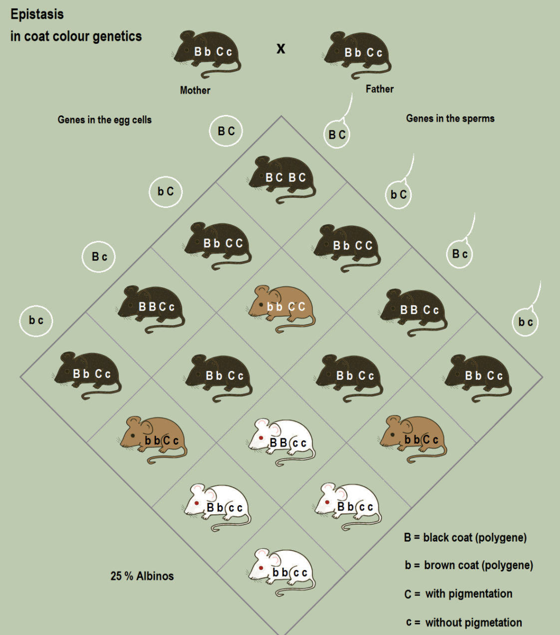
Identifying eQTLs is complicated by epistasis and pleiotropy, which introduce nontrivial genetic interactions. Epistasis occurs when the effect of a SNP on gene expression depends on the presence of other genetic variants, making it difficult to model simple SNP-expression relationships, see Figure 7.28. This can obscure true associations if not explicitly accounted for in statistical models. Pleiotropy, where a single SNP influences multiple genes or traits, further complicates eQTL discovery by creating indirect associations that may not reflect true causal regulatory relationships. These complexities highlight the challenge of interpreting eQTL results solely through single-variant associations, necessitating approaches that account for gene-gene and gene-environment interactions.
7.4.0.4 By the Way, eQTL Is Not the Only Type of QTL!
While eQTL studies focus on linking genetic variation to gene expression, quantitative trait locus (QTL) mapping extends beyond transcriptomics to investigate various molecular and phenotypic traits. In addition to eQTLs, other types of QTLs provide insights into the genetic regulation of different cellular processes.
One important class of QTLs is splicing QTLs (sQTLs), which identify genetic variants that influence alternative splicing patterns. These variants may affect exon inclusion, intron retention, or alternative polyadenylation sites, ultimately leading to differences in transcript isoforms. Splicing QTL studies are particularly relevant in diseases where aberrant splicing plays a critical role, such as neurological disorders and cancer.
Another type is chromatin accessibility QTLs (caQTLs), which link genetic variants to changes in chromatin openness, often measured using ATAC-seq. These QTLs help identify regulatory elements such as enhancers and promoters that may be modulated by genetic variation, affecting transcription factor binding and downstream gene expression.
Collectively, we call the set of all possible QTLs as xQTL, see Ng et al. (2017). (I know, this can sound like alphabet soup the very first time you learn about these.)
7.4.0.5 By the way… LLMs are also in this race.
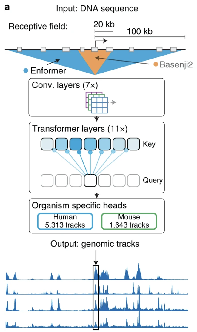
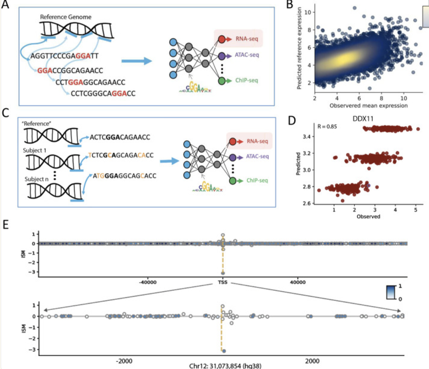
Recent advances in large language models (LLMs) have enabled the prediction of gene expression directly from raw DNA sequences, leveraging architectures such as transformers, convolutional neural networks (CNNs), and recurrent neural networks (RNNs), see Figure 7.29 and Figure 7.30. These models, trained on genomic sequences, learn complex regulatory grammar and sequence motifs to infer transcriptional activity. Unlike eQTL studies, which link genetic variants to expression using population-level variation, LLMs aim to predict expression from intrinsic sequence features, potentially identifying novel regulatory elements. This approach complements TWAS by offering a purely sequence-driven method to estimate gene expression, independent of population structure or linkage disequilibrium, enhancing our understanding of transcriptional regulation. See Sasse et al. (2023) for an overview.
7.5 Other (very large areas of cell biology) that perform multi-omic analyses involving genetics
The following are some of gigantic areas of genetics which span multiple omics that I’m doing a disservice to by simply summarizing as bullet points. (We’ll discuss phylogenetics briefly in [Section @ref(sec-natural_lineage)], which is another massive area.) The point is – if you really want to study a human disease, you’ll eventually need to learn genetics at point in your career (even if it’s not directly during your PhD or post-doc). It’s almost inevitable.
- Polygenic risk scores:
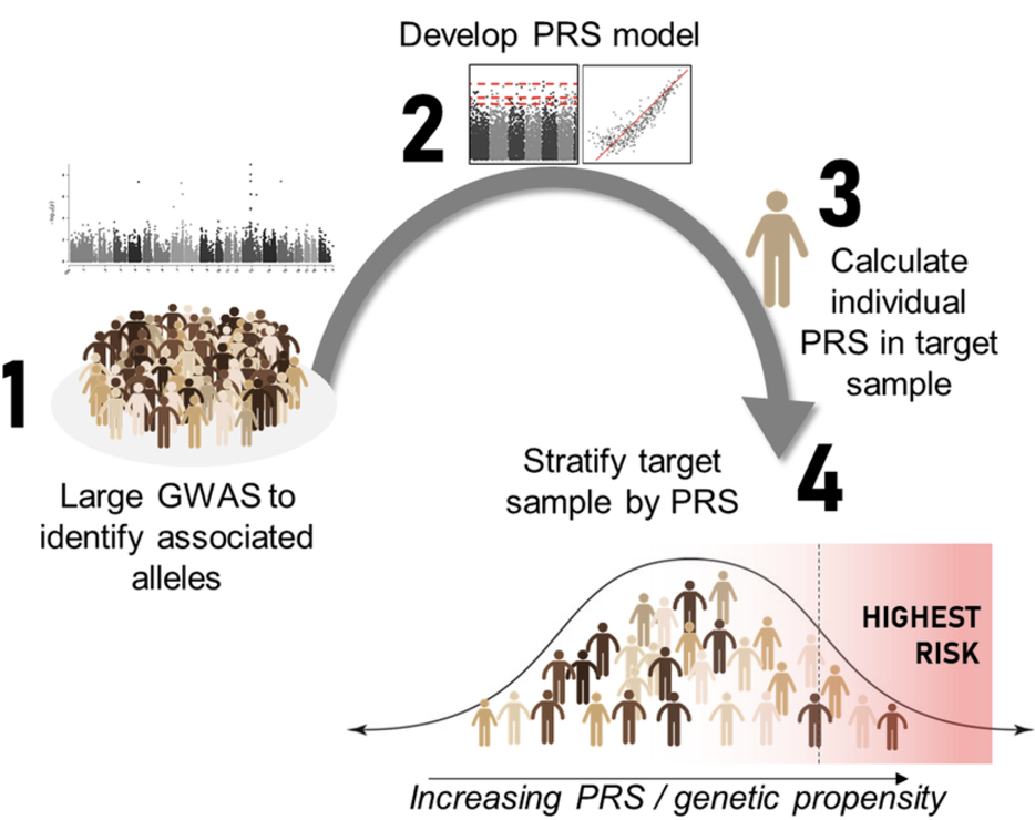
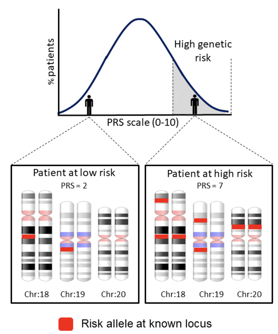
Polygenic risk scores (PRS) aim to quantify an individual’s genetic predisposition to a disease or trait by aggregating the effects of many common genetic variants identified from genome-wide association studies (GWAS). The biological goal of PRS is to develop predictive models that estimate disease susceptibility based on an individual’s genotype, providing a tool for early disease screening, personalized medicine, and risk stratification, see Figure 7.31 and Figure 7.32. PRS is particularly useful in complex diseases, where multiple genetic variants contribute small additive effects to disease risk.
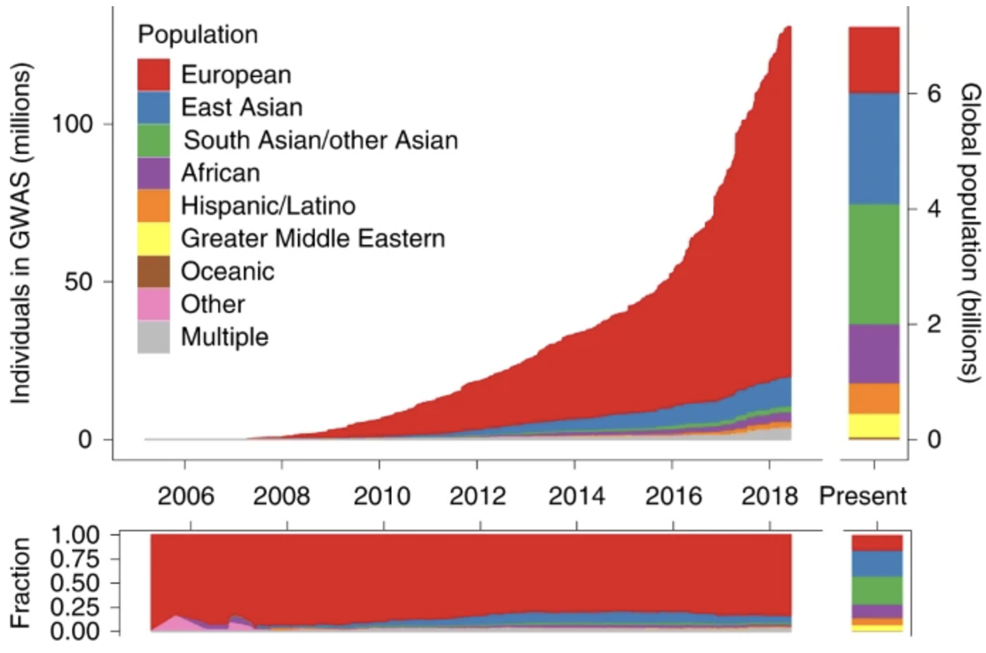
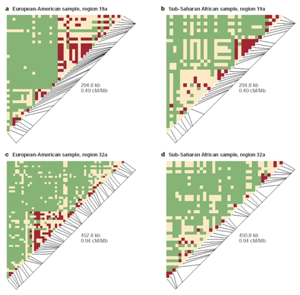
PRS construction relies on large GWAS datasets that provide summary statistics on variant-trait associations. The scores are computed by summing the weighted effects of risk alleles across the genome, often using computational tools like LDpred Privé, Arbel, and Vilhjálmsson (2020) and PRS-CS Ge et al. (2019). However, one of the biggest challenges in PRS research is population stratification and ethnicity bias. Since most GWAS studies have been conducted in individuals of European ancestry, PRS models trained on these datasets often fail to generalize well to non-European populations due to differences in allele frequencies and linkage disequilibrium (LD) patterns, see Figure 7.33 and Figure 7.34. Addressing this computationally is a huge area of current research. For an example of PRS for single-cell data, see scDRS M. J. Zhang et al. (2022).
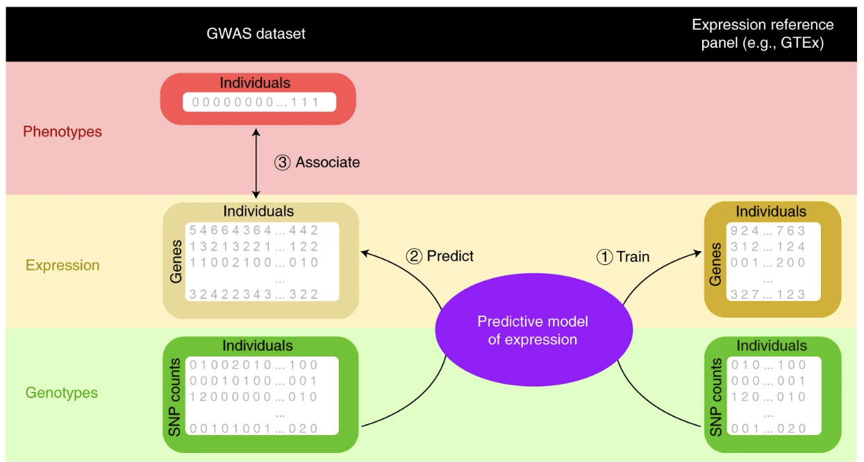
- Transcriptomic-wide association study (TWAS): A Transcriptome-Wide Association Study (TWAS) aims to identify genes whose expression levels are associated with complex traits and diseases by integrating genome-wide association study (GWAS) data with transcriptomic data. The biological goal of TWAS is to bridge the gap between genetic variation and gene expression to prioritize candidate causal genes that might drive disease susceptibility. In a overly simplistic sense, you can think of the following: \[ \text{GWAS:} \quad \text{SNP} \;\rightarrow\; \text{Disease phenotype} \] \[ \text{eQTL:} \quad \text{SNP} \;\rightarrow\; \text{Gene expression} \] \[ \text{TWAS:} \quad \text{Genetically predicted gene expression} \;\rightarrow\; \text{Disease phenotype} \] Unlike GWAS, which identifies loci associated with disease risk but does not directly implicate specific genes, TWAS infers putative gene-disease relationships by leveraging genetic regulation of gene expression. See Mai et al. (2023) for an overview.
The data required for TWAS includes GWAS summary statistics and expression quantitative trait loci (eQTL) datasets derived from bulk RNA-sequencing or single-cell RNA-sequencing studies. Typically, eQTL datasets are obtained from large-scale population-based biobanks like GTEx or UK Biobank. Common computational approaches used for TWAS include PrediXcan and FUSION, which estimate genetically predicted gene expression levels based on genotype data and test for associations with traits. However, TWAS has important caveats: it typically assume that genetically regulated gene expression effects are the primary driver of trait associations, which may not always be the case. Moreover, TWAS inherits any demographic limitations of GWAS and eQTL analyses, which means these results are often biased toward European ancestry populations due to data limitations. For an example of PRS for single-cell data, see scPredixcan Zhou et al. (2024).
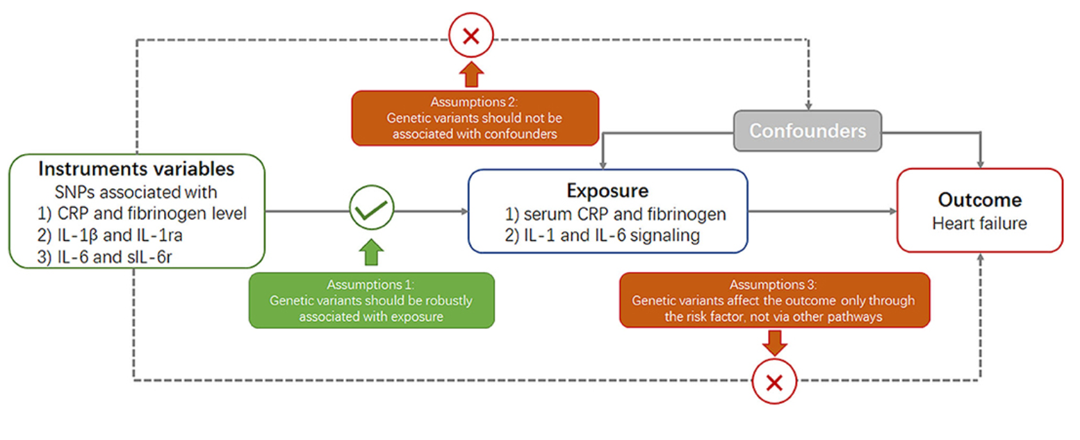
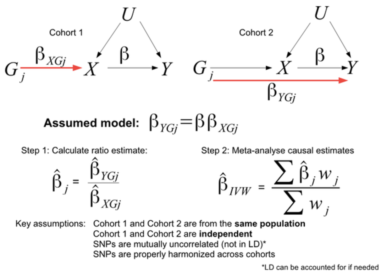
- Mendelian randomization: Mendelian Randomization (MR) is a statistical approach used to infer causal relationships between an exposure (such as gene expression, biomarker levels, or lifestyle factors) and an outcome (such as disease risk) by leveraging genetic variants as instrumental variables. The biological goal of MR is to overcome confounding and reverse causation issues that plague observational studies, making it a powerful tool for identifying causal risk factors for diseases. MR is particularly useful in prioritizing drug targets, as it can provide evidence on whether modifying a specific biomarker or gene expression level is likely to have a therapeutic effect.
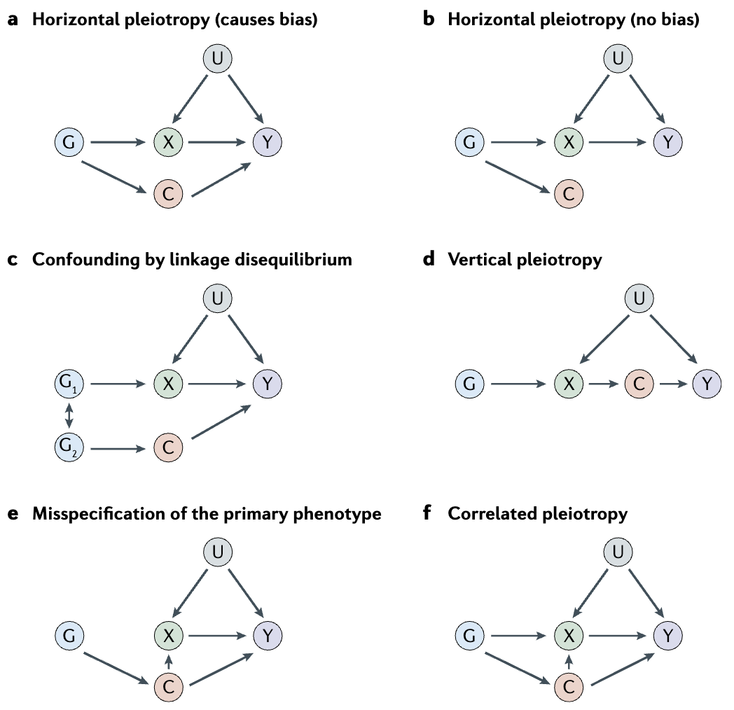
MR studies require genetic association data from large GWAS and eQTL datasets to identify genetic instruments that are robustly associated with the exposure of interest. The commonly used computational tools for MR analysis include MR-Egger Burgess and Thompson (2017), MR-PRESSO Verbanck et al. (2018), and TwoSampleMR Hartwig et al. (2016), which help detect and correct for pleiotropy and other biases. However, MR has several limitations. First, the validity of MR results depends on the assumption that the chosen genetic variants only influence the outcome through the exposure and not through other pathways (i.e., no horizontal pleiotropy), see Figure 7.36 and Figure 7.38. Additionally, weak instrument bias can occur when genetic instruments have small effect sizes, reducing statistical power. Because many complex traits are influenced by highly pleiotropic variants and gene-environment interactions, refining MR methodologies and integrating multi-omics data remains an active area of research.
7.6 Structural variation: Focusing on copy number variation
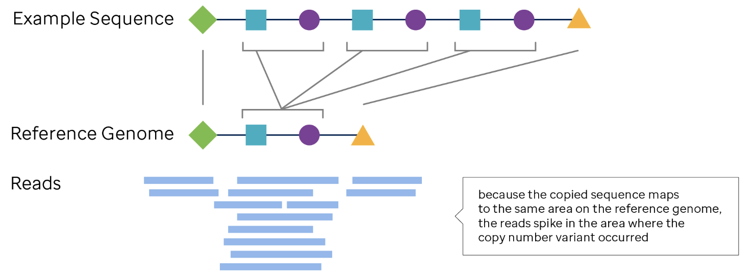
Copy Number Variation (CNV) refers to structural alterations in the genome that result in abnormal numbers of copies of one or more DNA segments. These can range from small events (a few hundred base pairs) to large events (millions of base pairs). CNVs can arise due to duplications, deletions, and, in rare cases, more complex rearrangements of genomic regions.
7.6.0.1 Importance of CNVs.
- Genetic diversity: CNVs are a major contributor to human genetic variation and can affect gene expression and phenotypic traits.
- Disease relevance: CNVs have been implicated in cancers, developmental disorders, autoimmune diseases, and more.
- Diagnostic value: Detection of CNVs can provide diagnostic and prognostic markers for clinical use.
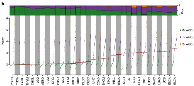
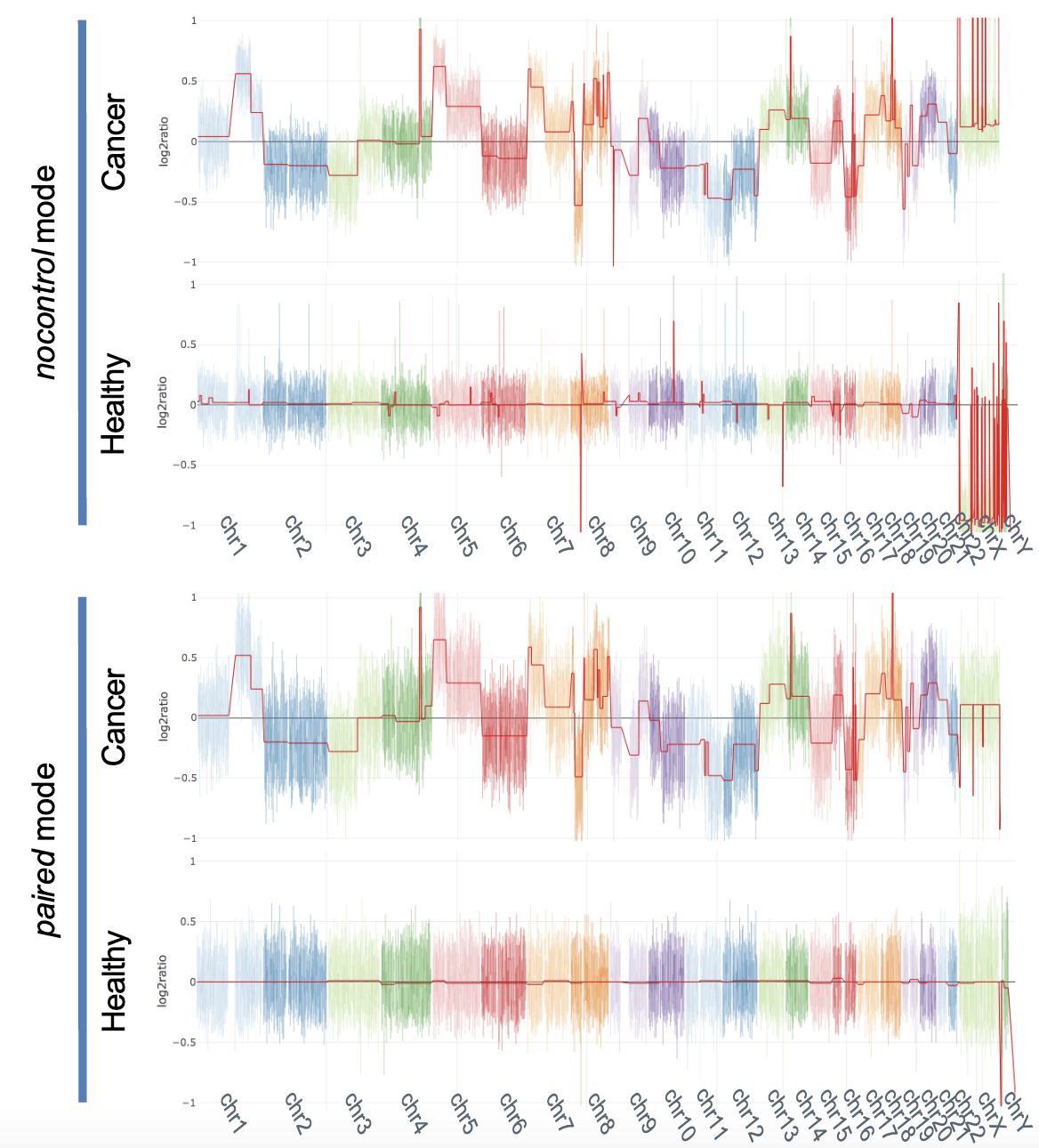
See Figure 7.42 on how copy number presents a strong signal in cancer. As an aside though, not all copy number events are necessarily deleterious. Copy number variation (depending on the region) can also be benign – see Erickson et al. (2022), Mihaylova et al. (2017).
In this set of notes, we focus on how CNVs are detected using sequencing data and the computational steps required to identify and interpret these variants.
7.6.0.2 Sequencing-based technologies for CNV detection, and single-cell variations
Single-cell sequencing of DNA enables the detection of copy-number variations (CNVs) at a single-cell resolution, offering insights into cellular heterogeneity, clonal evolution in cancer, and somatic mutations in various diseases. Unlike bulk sequencing, which averages signals across many cells, single-cell sequencing allows researchers to uncover rare and cell-specific genomic changes. The three main sequencing approaches—short-read sequencing, long-read sequencing, and whole-genome sequencing (WGS)—each have distinct advantages and challenges when applied to single-cell CNV detection.
Short-Read Sequencing (e.g. Illumina):
Short-read sequencing, commonly used in single-cell DNA studies, generates high-throughput data with read lengths of 50–300 bp. Due to the limited DNA in single cells, whole-genome amplification (WGA) is required, introducing variability in coverage. This approach enables profiling of thousands to millions of cells, making it scalable for large studies. However, the short read length limits the resolution of large or complex CNVs, particularly in repetitive regions.
Long-Read Sequencing (e.g. PacBio, Oxford Nanopore):
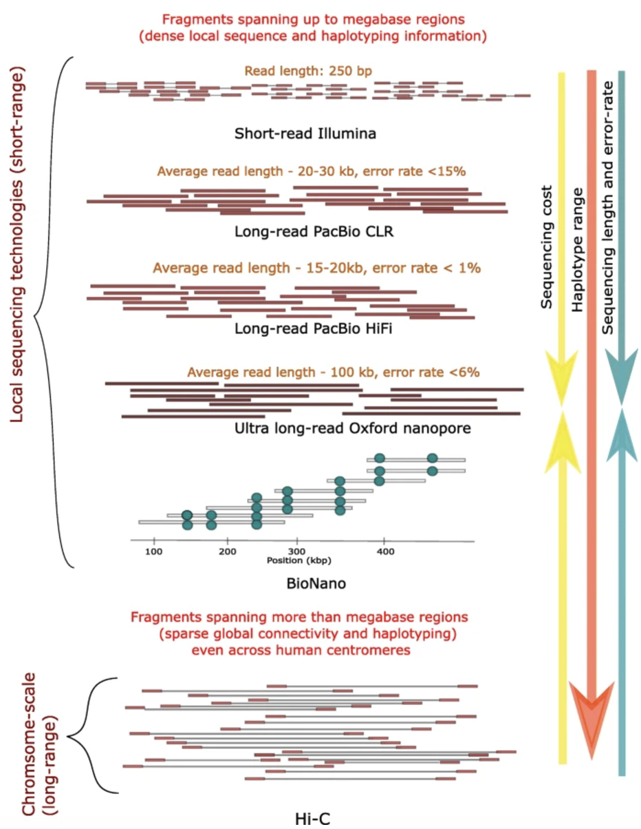
Long-read sequencing generates reads spanning several kilobases, allowing direct observation of large CNVs and structural rearrangements. Unlike short-read methods, long reads can span entire CNV breakpoints and enable haplotype phasing, providing insights into allele-specific genomic alterations. While lower in throughput, this approach improves the resolution of highly rearranged regions. See Figure 7.43.
Whole Genome Sequencing (WGS) in General:
Single-cell WGS provides an unbiased approach to detecting CNVs across the entire genome without prior assumptions about affected regions.
Because of the high cost of sequencing, single-cell WGS is often performed at relatively low coverage (e.g., 0.1–10x), which can impact the sensitivity and resolution of CNV detection. Additionally, single-cell WGS is prone to artifacts introduced by whole-genome amplification, sequencing errors, and allelic dropout events, necessitating advanced bioinformatics methods to correct for these biases.
WGS generates vast amounts of data, requiring significant computational resources and careful handling of sequencing artifacts, but remains the most comprehensive method for CNV analysis.
The choice of sequencing technology depends on the research question, budget, and required resolution of CNV detection. To compare the three archetypical approaches:
| Feature | Short-Read (Illumina) | Long-Read (PacBio/Nanopore) | WGS (Whole-Genome) |
|---|---|---|---|
| Resolution | High for small CNVs | High for large CNVs | Genome-wide |
| Scalability | High (many cells) | Lower (limited throughput) | Moderate |
| Cost | Lower per base | Higher per base | High for large cohorts |
| Read Length | 50–300 bp | Thousands of bp | Short or long reads |
| Biases | WGA bias | Higher per-base error | Amp. and dropout artifacts |
7.6.0.3 Computational Steps in CNV Analysis
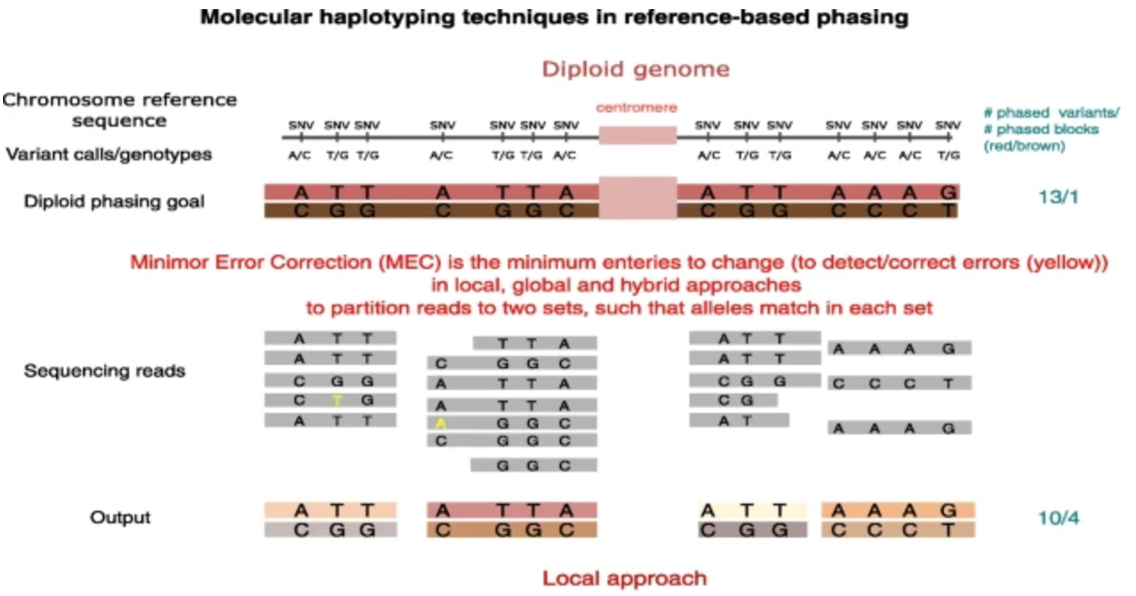
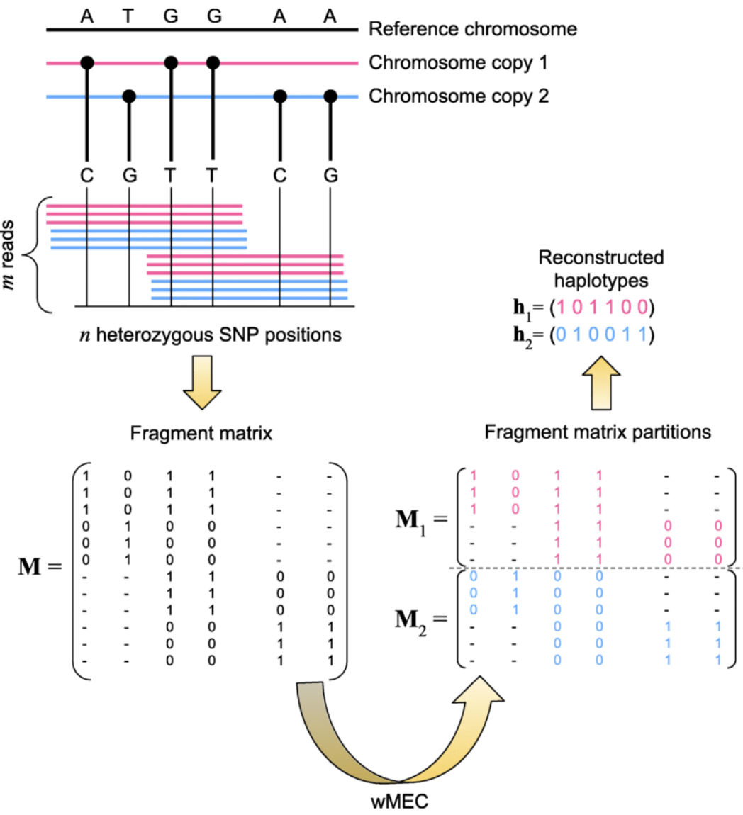
The detection of copy-number variations (CNVs) from sequencing data requires multiple computational steps, each of which contributes to the accuracy and reliability of CNV calls. While some steps are essential, others are optional or depend on the specific research question and available data. The main stages of CNV detection include preprocessing and quality control, mapping to a reference genome, haplotype phasing, and variant calling.
Some note about terminology: germline and somatic describe the biological origin of CNVs, while karyotyping is a method for detecting CNVs (mainly large ones).
Germline CNVs are inherited variations present in all cells of the body, including reproductive cells (sperm and egg).
Somatic CNVs arise during a person’s lifetime and are not inherited; they occur in specific tissues, often as a result of disease processes such as cancer.
Preprocessing and Quality Control:
Before analyzing sequencing data for CNVs, raw sequencing reads must undergo quality control and preprocessing to remove technical artifacts and improve downstream analysis accuracy. The first step is a raw data quality check using tools such asFastQC, which assesses read quality, adapter contamination, and potential sequencing artifacts. If necessary, trimming and filtering may be applied to remove low-quality reads and adapter sequences, ensuring that only high-quality data is used for subsequent analysis. Although trimming and filtering are optional, they are often beneficial for improving read alignment and overall variant detection accuracy.Mapping to a Reference Genome:
After preprocessing, sequencing reads must be aligned to a reference genome to determine their genomic positions. The choice of aligner depends on the sequencing technology used, with commonly used tools includingBWAandBowtie2for short-read sequencing andminimap2for long-read sequencing. Once aligned, the output is stored in a sorted and indexedBAMfile, which serves as the primary input for CNV detection and other genomic analyses. Proper alignment is crucial, as errors in mapping can introduce biases in CNV calling.Haplotype Phasing (Optional):
Haplotype phasing is an optional but useful step in CNV analysis that determines which genetic variants co-occur on the same chromosome copy. In the context of CNV calling, phasing is particularly valuable when investigating whether duplications or deletions are located on the same haplotype. This information can provide insights into the inheritance patterns of CNVs and their potential functional effects. Tools such asWhatshapandHapCUT2can be used to perform haplotype phasing based on read alignment data, helping to refine CNV interpretation.
Variant Calling and CNV Detection Inputs:
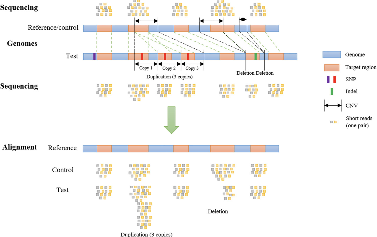
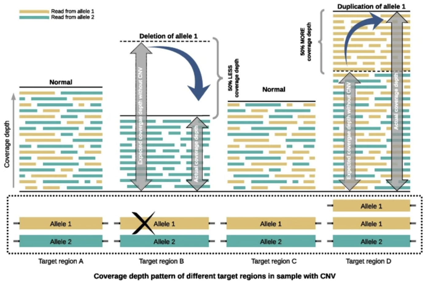
CNV detection relies on multiple sources of information extracted from sequencing data. One key input is single nucleotide polymorphism (SNP) calls, which are generated using tools likeGATKandbcftools. SNP data can aid CNV detection by identifying allele frequency shifts, refining CNV breakpoints, and confirming copy-number gains or losses. Additionally, read depth calculation is a fundamental step in CNV calling, as CNVs typically manifest as regions with increased or decreased sequencing coverage. Tools such asCNVnatorfor short-read sequencing anddeepToolsfor depth-based analysis provide means to quantify read depth across genomic windows, facilitating CNV identification.Copy number detection algorithms:
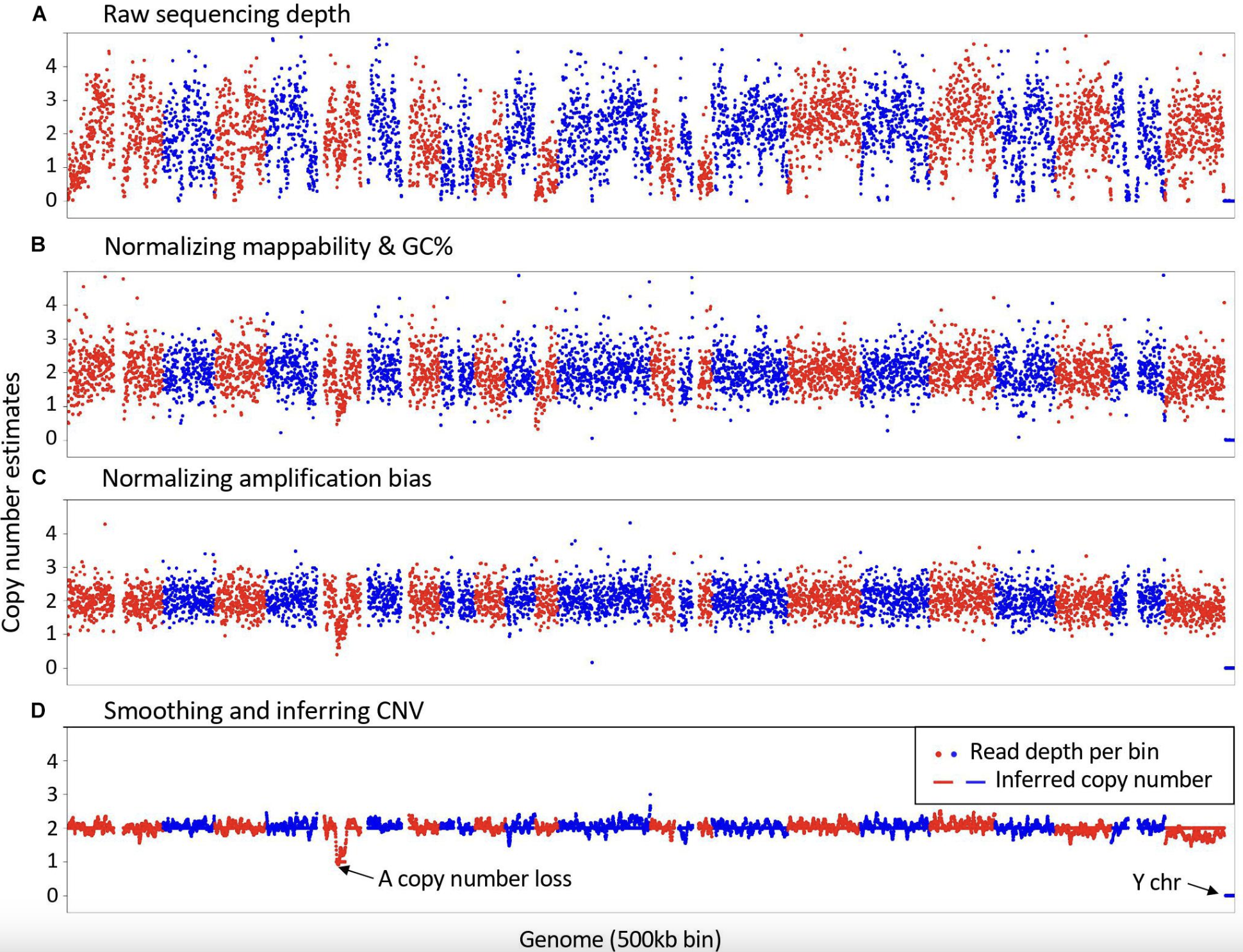
CNV detection methods broadly fall into two categories: window-based coverage analysis and event-based methods. In window-based approaches, the genome is partitioned into fixed-size bins (e.g., 1 kb or 10 kb), and read coverage within each bin is compared to an expected distribution. Hidden Markov models (HMMs) and segmentation algorithms are then used to identify regions with significantly higher or lower coverage, indicative of duplications or deletions. Event-based methods, in contrast, focus on identifying breakpoints in sequencing coverage or read-pair orientation, leveraging structural changes across multiple reads to confirm CNV events.Establishing a “Control” Baseline:
To distinguish true CNVs from technical artifacts, a reference baseline is often established using a “panel of normals,” which consists of aggregated sequencing data from healthy individuals. This helps correct for systematic biases and variability in coverage. In cases where a matched normal sample from the same individual is available, such as in tumor-normal studies, it serves as an optimal reference for identifying somatic CNVs. Regions with significantly elevated or reduced coverage relative to the control are flagged as potential duplications or deletions.
- Correcting biases and finalizing CNV calls:
Several sources of bias must be accounted for in CNV analysis to improve accuracy. GC content bias occurs because regions with extreme GC composition may be preferentially over- or under-sequenced, affecting coverage estimates. Batch effects arise due to differences in sequencing runs, library preparation protocols, or platform variability, necessitating normalization across datasets. Mappability issues, particularly in repetitive or low-complexity genomic regions, can lead to ambiguous read alignments and false-positive CNV calls. Many CNV detection pipelines incorporate bias correction strategies, such as GC normalization and read-depth smoothing, to improve reliability in final CNV calls.
See Masood et al. (2024), L. Zhang et al. (2019) for benchmarking across various methods for CNV.
See Gordeeva et al. (2021) for a review on whole exome sequencing.
7.6.1 A quick note on the reference genome
When doing structural variation analyses, there is an inherent question of “what genome are you comparing against.” This is natural, as CNV is (loosely speaking) about “deviations from the typical genome,” so we need to think hard about what we are referring to when we say “typical genome.”
While simplistic in explanation, there are multiple problems stemming from this pipeline. The main issue stems from the fallacy of this notion of a “reference” genome. As stated in Ballouz, Dobin, and Gillis (2019), there are many possible pitfalls of relying on a reference genome.
As a quote from Ballouz, Dobin, and Gillis (2019):
Remark: (The reference genome is not a ‘healthy’ genome, ‘nor the most common, nor the longest, nor an ancestral haplotype’.)
Efforts to fix these ‘errors’ include adjusting alleles to the preferred or major allele or the use of targeted and ethnically matched genomes.
So really, the reference genome is simply an “addressing system” that many researchers can agree upon to get reproducible findings. Unsurprisingly, due to our understanding of CNV, we do not simply “count” how far along from the “start” of the chromosome we are (say, in terms of kb). This is because any CNV would shift our count. Instead we must first rely on a reference genome.
Certainly, changing the reference genome can potentially change the results quite substantially. See papers such as Pan et al. (2019) and Wong et al. (2020).
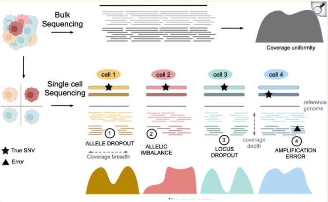
7.6.2 Challenges of collecting “single-cell DNA” sequencing data
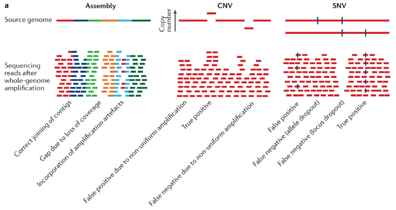
Single-cell DNA sequencing, whether whole-genome or whole-exome, must contend with the fact that each cell contains only two copies of the genome, making any loss of genetic material “permanent.” This inherently low starting material magnifies several issues:
- Allele (locus) dropout: The random loss or failure to amplify one allele, resulting in incomplete or missing data for certain loci.
- Allelic imbalance: Unequal amplification efficiency of different alleles, which can skew variant calling and downstream analyses.
- Amplification error: The polymerase-mediated amplification steps can introduce additional errors or biases, confounding true biological variation.
See Figure 7.48 and Figure 7.49 for examples, and the citations mentioned there. This is a rapidly evolving field. For an example of technology that is performing multiome sequencing of RNA and WGS DNA, see scONE-seq Yu et al. (2023). For an example of diagonal integration between scRNA-seq and scDNA-seq, see Edrisi et al. (2023). See Hård et al. (2023) for how long-read sequencing is transforming the prospects of WGS DNA sequencing at single-cell resolution.
7.6.3 Studying single-cell copy-number variation using scRNA-seq data
7.6.3.1 A typical choice: CopyKAT.
Copy number karyotyping of aneuploid tumors (CopyKAT) Gao et al. (2021) is a Bayesian segmentation approach designed to infer genomic copy number profiles from single-cell RNA sequencing (scRNA-seq) data. This method distinguishes aneuploid tumor cells from diploid stromal and immune cells, enabling the characterization of clonal substructure within tumors. CopyKAT operates by ordering genes based on genomic coordinates, defining diploid controls, segmenting chromosomal regions, and clustering cells into subpopulations based on their copy number profiles.
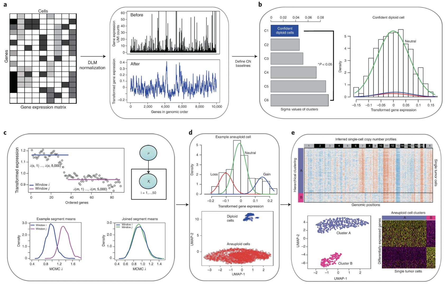
- Modeling scRNA-seq Data for Copy Number Estimation.
Given a gene expression matrix \(X\) with rows representing genes and columns representing cells, CopyKAT begins by transforming raw unique molecular identifier (UMI) counts to stabilize variance. The log-Freeman–Tukey transformation is applied:
\[ X' = \log\left(\sqrt{X} + \sqrt{X+1}\right) \]
To smooth outliers and reduce noise, polynomial dynamic linear modeling (DLM) is applied, resulting in a denoised expression matrix that captures genomic trends while mitigating single-cell technical variability.
- Identifying Diploid Control Cells.
A subset of normal diploid cells is needed to define the baseline expression profile for copy number inference. CopyKAT achieves this through clustering of the cells into 6 clusters, and then a Gaussian mixture model (GMM) is performed for the median expression for a cluster3. This GMM is used to determine a mixture of 3 Gaussians (to represent lower, baseline, or higher copy number.) The cluster with the lowest variance across genes in the GMM model is designated as the set of confident diploid cells, assuming their gene expression patterns reflect a neutral (2N) copy number state.
- Defining Copy Number Breakpoints.
Chromosomal breakpoints are inferred through a Poisson-gamma model combined with Markov Chain Monte Carlo (MCMC) sampling.
As a side-note, MCMC methods are widely used in CNV analysis because CNV segmentation involves inferring hidden states (copy number gains/losses) from noisy data.
This is great for CNV analyses since the copy number state of a genomic window is dependent on the state of adjacent windows.
Determining where a CNV starts and ends involves estimating hidden parameters, such as segment boundaries and copy number values.
MCMC helps solve these problems by iteratively sampling from the posterior distribution of possible segmentations.
To do this, CopyKAT first computes the median gene expression for each cluster of cells. Then, for a chromosome, it bins all the genes (in order along that chromosome), and models the median gene expression among all the genes in this bin with the model:
\[ X_{kj} \sim \text{Poisson}(\lambda_{kj}), \quad \lambda_{kj} \sim \text{Gamma}(\alpha_{kw}, \beta_{kw}), \quad \text{for bin $w$ containing gene $j$} \]
where \(X_{kj}\) represents the original gene counts for gene \(j\) in cluster \(k\), and \(\alpha_{kw}\) and \(\beta_{kw}\) are parameters for this particular genomic bin \(w\) (containing gene \(j\)) and cell cluster. CopyKAT starts with bins with equal number of genes in this chromosome (again, in order along the chromosome).
The posterior mean for the genomic bin is computed, and a Kolmogorov–Smirnov (KS) test is used to determine if adjacent regions should be merged. The final breakpoints are determined iteratively by pooling results across single cells, establishing consensus boundaries of copy number variation.
- Detecting Deviations from Controls.
Once a reference baseline is established, CopyKAT computes relative gene expression deviations by subtracting the median expression values of the diploid control cells:
\[ Z_{ij} = X'_{ij} - \text{median}(X'_{\text{diploid},j}) \]
for cell \(i\) and genomic segment \(j\), where the above median is across all the genes in the chromosome.
These deviations serve as the basis for segmenting chromosomal regions into three copy number states: loss, neutral, and gain.
- Clustering Cells Based on Copy Number Profiles.
Hierarchical clustering is applied to group cells based on their copy number profiles. The clustering is performed using Ward’s linkage and Euclidean distance. Two main clusters are identified: one representing normal diploid cells and the other capturing aneuploid tumor cells. Within the aneuploid cluster, further subdivision is performed to delineate distinct tumor subpopulations with unique copy number alterations.
7.6.3.2 A brief note about other approaches.
There are a lot of scRNA-seq methods to infer CNVs. See Chen et al. (2024) for a benchmarking.
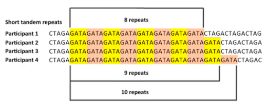
7.6.4 Other fascinating research on structural variation: Short tandem repeats
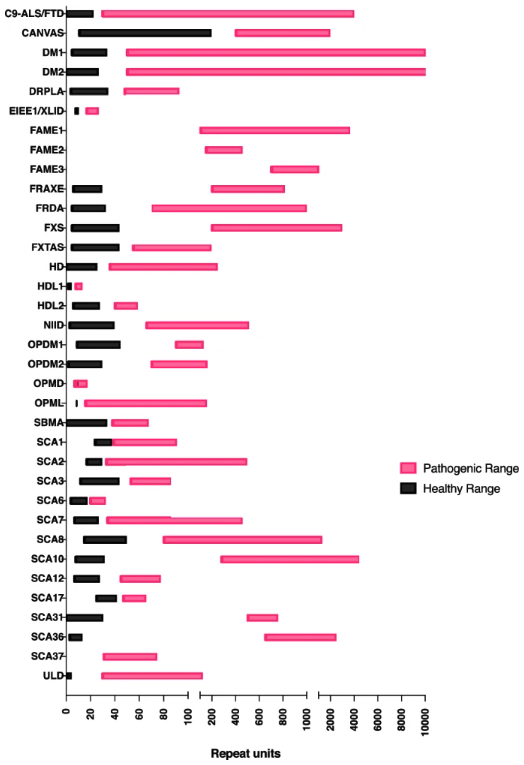
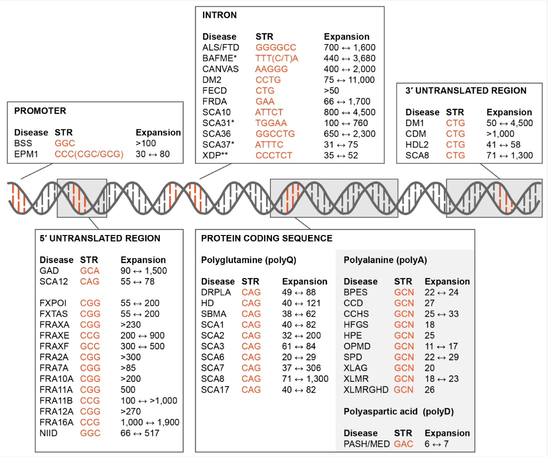
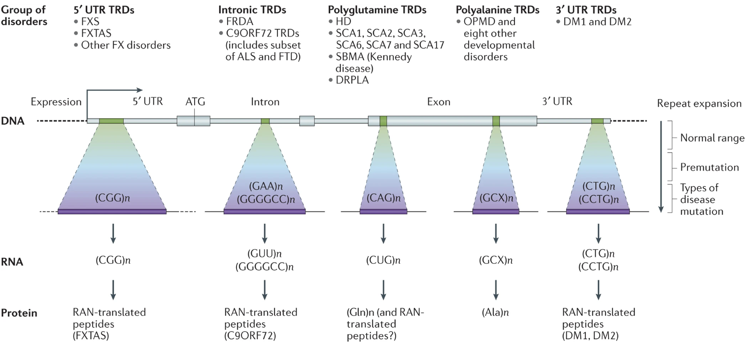
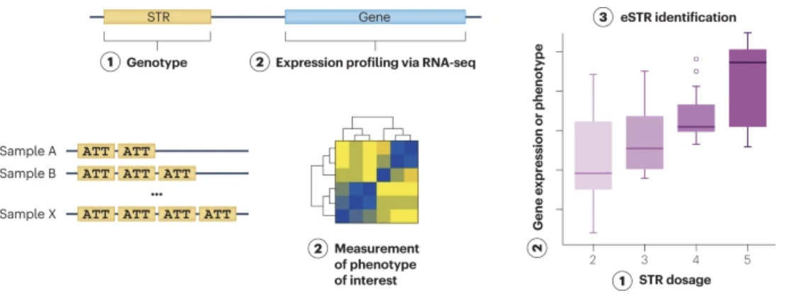
Short Tandem Repeats (STRs) are short, consecutive sequences of nucleotides, typically ranging from two to six base pairs, that are repeated multiple times in a head-to-tail fashion, see Figure 7.51 and Figure 7.52. These repeated segments can vary in length among different individuals, making STRs a valuable marker for genetic identification and population studies. They occur throughout the genome and often exhibit high mutation rates, which contribute to genetic diversity, see Figure 7.53.
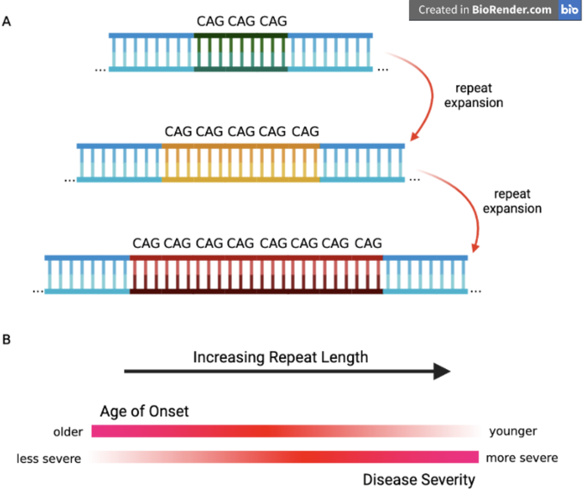
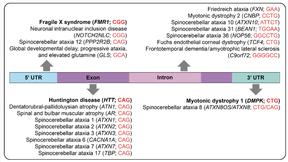
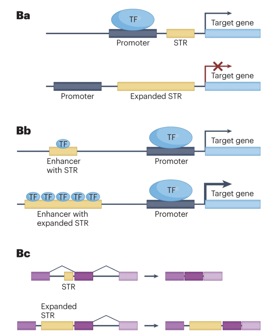
STRs are biologically significant because they can influence gene expression and genomic stability. Changes in the number of repeat units can alter regulatory regions or disrupt coding sequences, leading to variations in protein function or levels of gene expression. In some cases, expanded STRs are associated with disease mechanisms, such as those underlying disorders like Huntington’s disease or Fragile X syndrome.
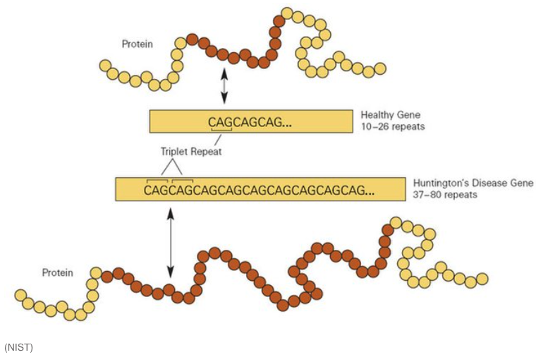
Clinically, studying STRs can aid in understanding the genetic basis of certain disorders and in diagnosing conditions caused by abnormal repeat expansions, see Figure 7.54. One prominent example is Huntington’s disease, which results from expansions of a CAG repeat in the HTT gene, see Figure 7.56. This leads to an elongated polyglutamine tract in the huntingtin protein, ultimately causing neuronal dysfunction and cell death. STR research, especially when coupled with single-cell sequencing approaches, has provided new perspectives on how expansions arise and progress at the cellular level. By revealing subtle, cell-to-cell differences in repeat length, researchers can better understand disease onset, severity, and variability in progression, opening up avenues for more targeted therapies and personalized disease management.
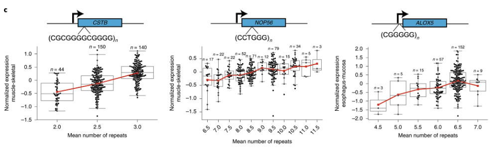
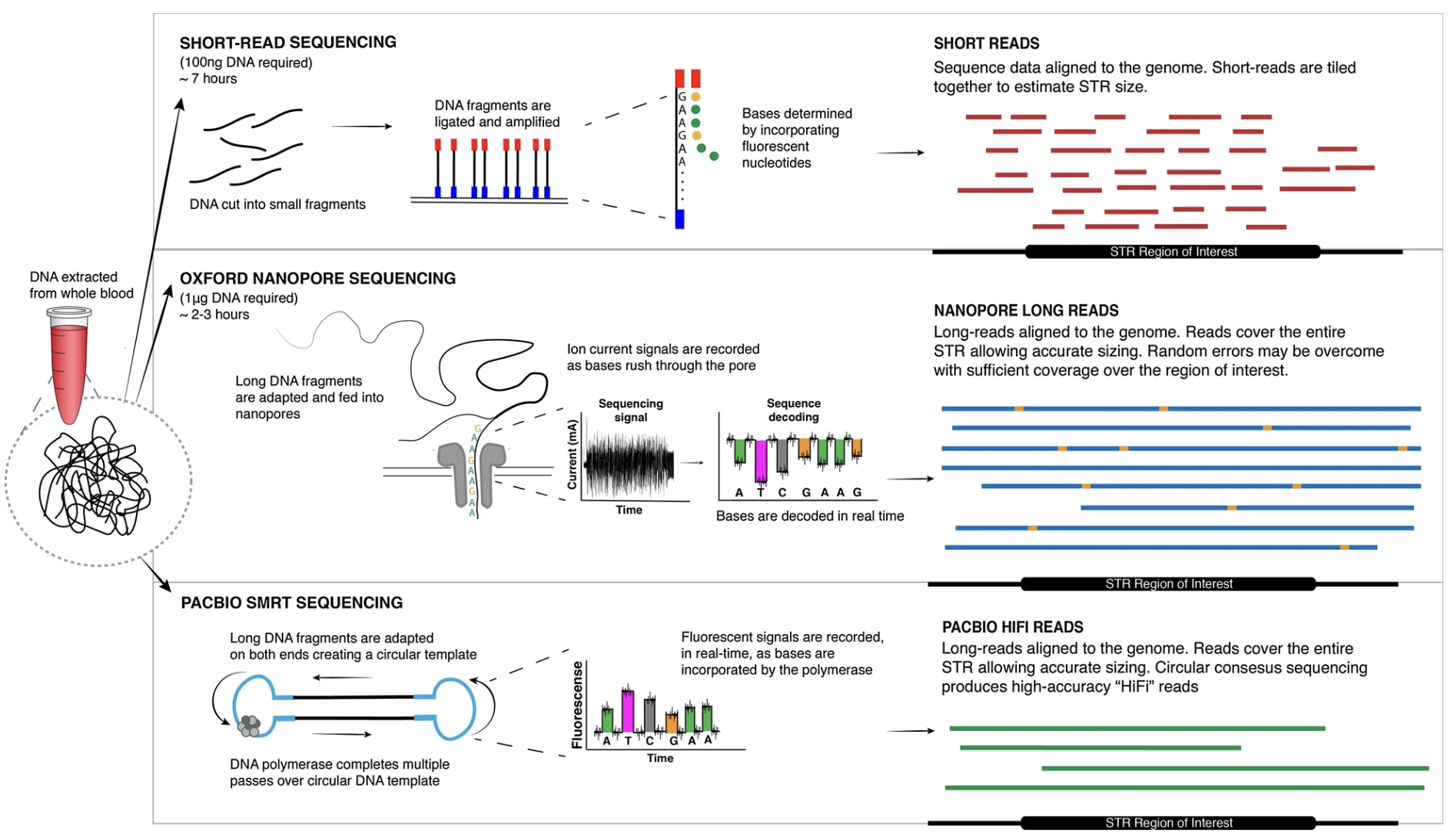
Modern analyses of Short Tandem Repeats (STRs) increasingly utilize various forms of sequencing data to pinpoint the location of these repeats and assess their potential functional roles, see Figure 7.57. Whole-genome sequencing (WGS) and targeted sequencing are often employed to identify both the presence and exact length of STR loci. Using short-read sequencing, computational methods can detect the boundaries and expansions of repeats by aligning reads to a reference genome. This enables genome-wide surveys of repeats in large cohorts, allowing researchers to correlate specific repeat expansions or contractions with phenotypic traits or disease states, see Figure 7.58. In parallel, long-read sequencing platforms, such as those provided by Pacific Biosciences or Oxford Nanopore Technologies, facilitate the direct observation of longer repeats and complex regions that may be challenging to resolve with short reads, see Figure 7.62. By integrating data on the repeat location, length, and local genomic context, researchers can infer the putative functional impacts, such as disruptions to regulatory regions, alterations in protein-coding sequences, or other mechanisms by which STRs may influence gene expression and disease susceptibility, see Figure 7.60.
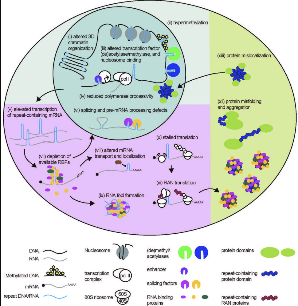
Short Tandem Repeats (STRs) are a hot topic in current genomics research because of their significant variability, functional importance, and direct implications in numerous neurological and developmental disorders. While advances in sequencing technology have enhanced our ability to detect and quantify these repeats, understanding their mechanistic roles in disease remains challenging. One major gap is the development of computational methods that rigorously map variations in STR length and composition to downstream biological processes, enabling a causal understanding of how specific repeat expansions contribute to pathogenesis. (We’re scanning billions of base pairs for each person (and possibly each cell) to find these STRs!) Until more sophisticated analytical pipelines and larger, well-characterized datasets are available, significant questions remain about how best to translate STR findings into actionable clinical insights.
See Chintalaphani et al. (2021) for tables of which STRs have been discovered to be associated with which diseases. See Tanudisastro et al. (2024), Hannan (2018) for more details on how STR occur, what their functional role is, and how they are studied.
See https://en.wikipedia.org/wiki/Directionality_(molecular_biology) and https://en.wikipedia.org/wiki/Sense_(molecular_biology).↩︎
To review, the Viterbi algorithm (https://en.wikipedia.org/wiki/Viterbi_algorithm) outputs the most likely sequence of underlying copy number profiles across the chromosome given the sequencing reads of each bin.↩︎
This is their
baseline.norm.clfunction, see https://github.com/navinlabcode/copykat/blob/master/R/baseline.norm.cl.R.↩︎