8 Single-cell CRISPR editting
8.1 Basics of how CRISPR works
The CRISPR-Cas system1 is a powerful genome-editing technology that allows for precise modifications of DNA in a wide range of biological systems. Originally derived from the bacterial adaptive immune system, CRISPR-Cas9 has been repurposed for genetic engineering by using a guide RNA (gRNA) to direct the Cas9 nuclease to a specific genomic locus for targeted DNA cleavage. This section discusses how CRISPR is performed in the wet lab, different functional applications of CRISPR, and how CRISPR-based perturbations are analyzed in single-cell gene expression studies.
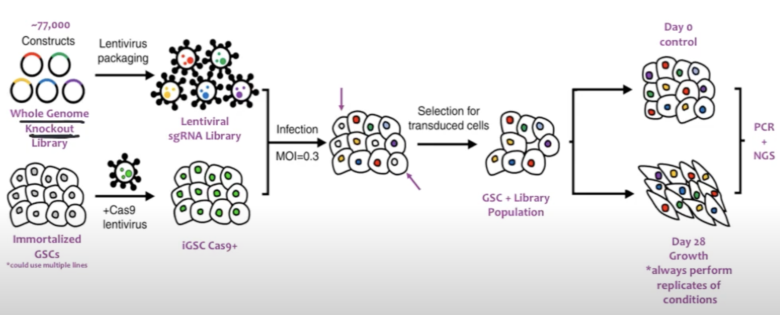
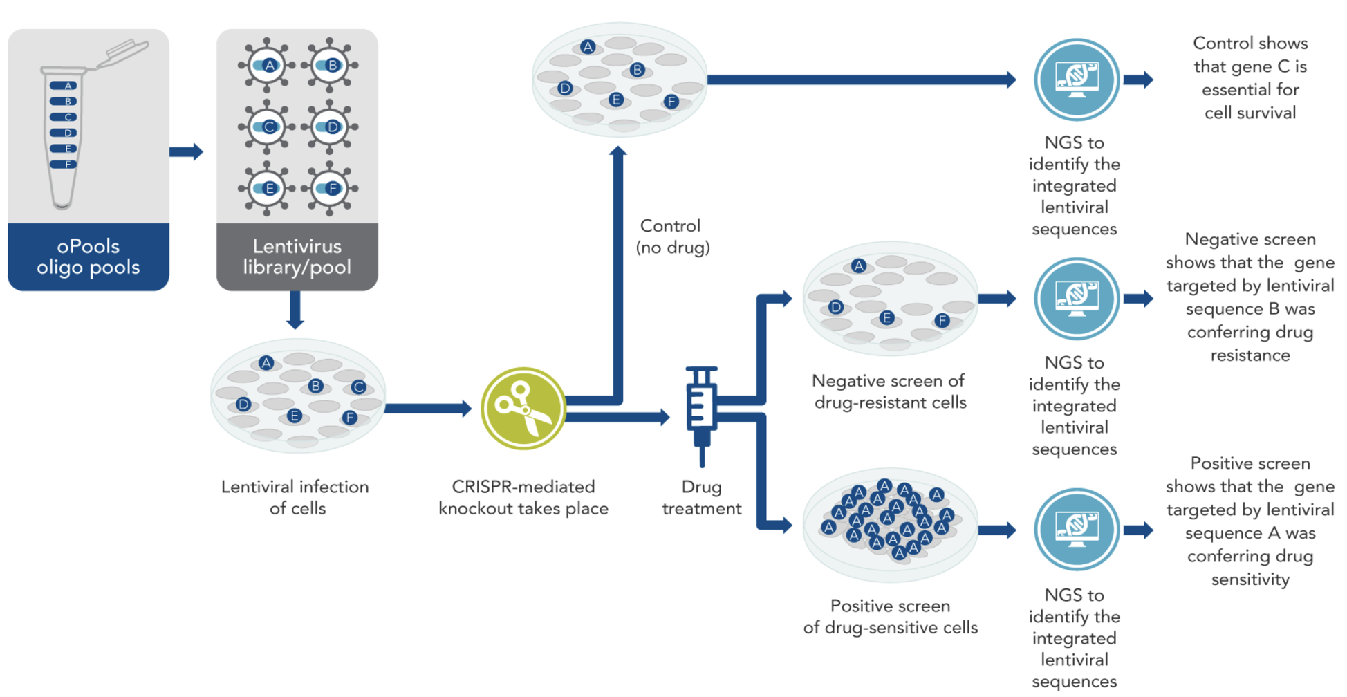
In a typical CRISPR screen experiment (mainly a CRISPR knockout), a library of lentivirus-packaged guide RNAs is introduced into cells under conditions designed to infect each cell with only one or a few sgRNAs (single guide RNA), see Figure 8.1 and Figure 8.2. After selection to ensure stable integration, the cells are subjected to a particular stimulus such as drug treatment or other environmental challenge. Researchers then track the abundance of each sgRNA at the start and after the stimulus (for example, at day 0 and day 28) through next-generation sequencing. By comparing which sgRNAs become enriched or depleted, it is possible to discover genes essential for viability, pathways governing drug resistance, or other critical biological functions relevant to the phenotype under study, see Figure 8.3.
Typical components of a CRISPR mechanism.
Cas9 protein: A DNA endonuclease that recognizes and cuts target DNA specified by the guide RNA; variations include nuclease-deactivated (dCas9) or nickase Cas9 for alternative applications. Other CRISPR-associated proteins like Cas12a (Cpf1), Cas13, or dCas9 (dead Cas9) can expand the range of target sequences, have different PAM requirements, or allow for gene regulation without cutting DNA.
Cas9 may bind sites with partial sequence complementarity, resulting in unintended cuts — this is called “off-target effects.” Various strategies (e.g., high-fidelity Cas9 variants, improved gRNA design) help minimize these effects.Guide RNA (gRNA): A customizable RNA sequence that directs Cas9 to the desired genomic locus; variations include single-guide RNA (sgRNA) and dual-RNA formats depending on the experimental design.
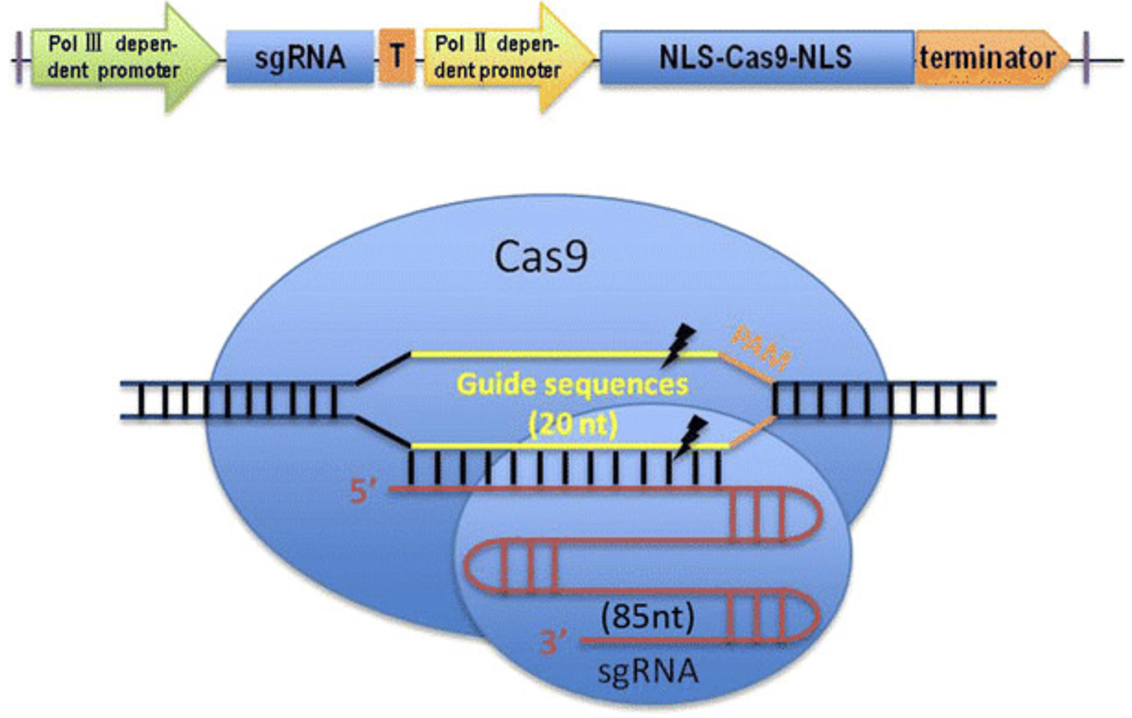
To streamline CRISPR-Cas9 applications in genetic engineering, scientists have designed a synthetic fusion of crRNA and tracrRNA into a single-guide RNA (sgRNA). This chimeric RNA retains both the target-specific recognition (crRNA component) and Cas9-binding function (tracrRNA component) but simplifies the system by reducing the number of necessary molecules. sgRNAs are commonly used in research and therapeutic applications due to their ease of design and efficiency in genome editing.- crRNA (CRISPR RNA): A short RNA sequence that is complementary to the target DNA and provides sequence specificity for Cas9 binding. This is typically 20 nucleotides long.
- tracrRNA (Trans-activating CRISPR RNA): A structural RNA that base-pairs with the crRNA and interacts with Cas9 to activate its nuclease function.
In this system, the crRNA and tracrRNA must form a duplex to guide Cas9 to the target sequence, which then leads to DNA cleavage.
Multiple guide RNAs can be delivered simultaneously to target different loci at once, enabling complex genome-scale screens or combinatorial gene perturbations. Computational tools help optimize sgRNA sequences to maximize on-target efficiency while minimizing off-target effects. Chemically modified guide RNAs can improve stability and efficiency in vivo.- crRNA (CRISPR RNA): A short RNA sequence that is complementary to the target DNA and provides sequence specificity for Cas9 binding. This is typically 20 nucleotides long.
PAM (Protospacer Adjacent Motif): A short DNA sequence adjacent to the target region that is essential for Cas9 to recognize and bind to DNA. The PAM sequence is typically “NGG” (where “N” represents any nucleotide, and “GG” is required). Without the correct PAM sequence, Cas9 cannot efficiently bind or cut the DNA, ensuring some level of specificity in genome editing. Different Cas9 variants have evolved or been engineered to recognize alternative PAM sequences, which offer broader targeting possibilities with reduced off-target effects. The cut typically happens 3 base-pairs upstream of the PAM on the target strand (i.e., in the 5′ direction).
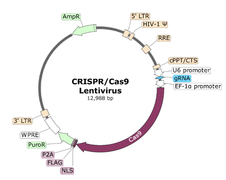
Lentivirus: Lentiviruses are widely used as viral vectors for delivering CRISPR components into cells (variations include different promoters, packaging systems, and envelope proteins to optimize transduction efficiency), particularly for experiments requiring stable and long-term expression of Cas9 and guide RNAs. Since many cell types are difficult to transfect using conventional methods, lentiviral transduction provides an efficient way to introduce CRISPR machinery into a broad range of cell types, including non-dividing and primary cells.
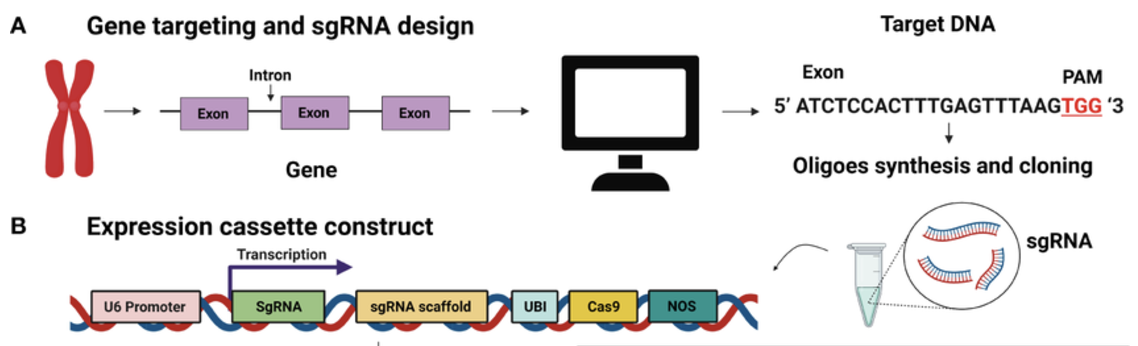
What is delivered to cells? (See Figure 8.4 for the construction and architecture of the lentiviral vector.)
- Cas9 expression construct: A lentiviral vector encoding the Cas9 nuclease under a suitable promoter. In some systems, inducible promoters (e.g., doxycycline-inducible) are used to control Cas9 activity.
- Guide RNA (gRNA) expression construct: A separate lentiviral vector encoding the guide RNA sequence under a promoter to ensure efficient transcription.
- Selection markers: Often, antibiotic resistance genes or fluorescent markers are included to facilitate selection of successfully transduced cells.
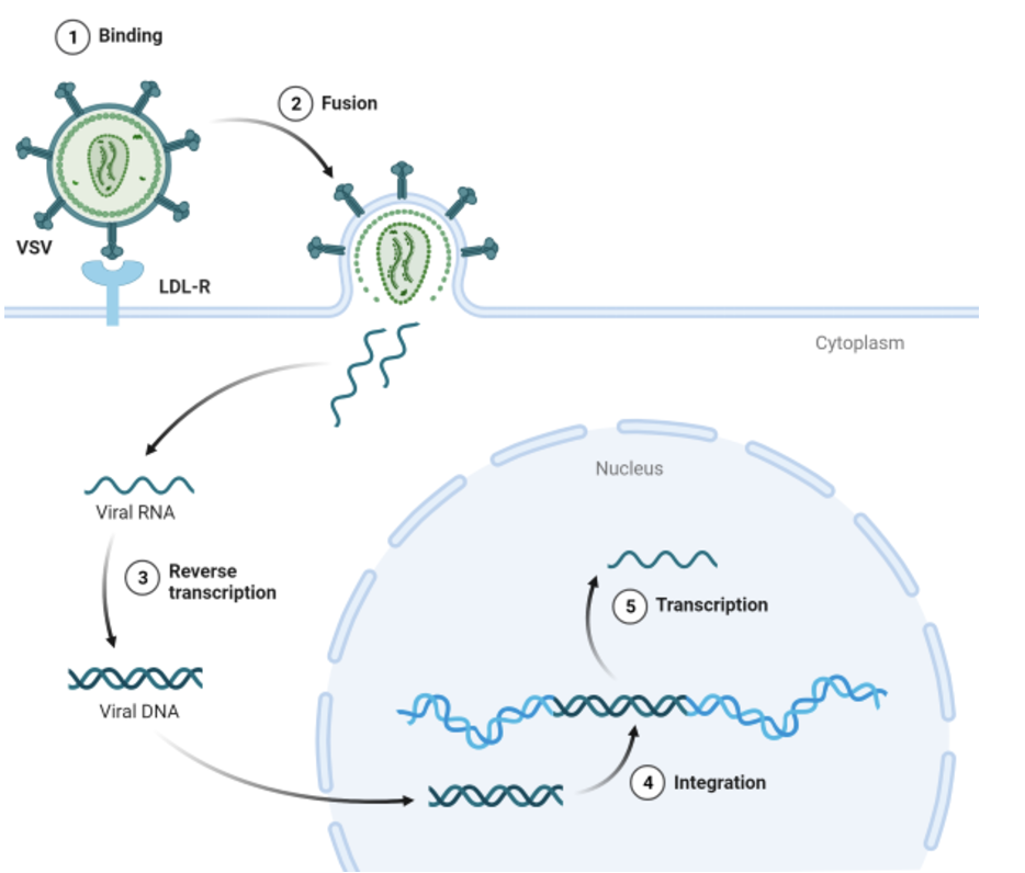
Lentiviral delivery is essential for CRISPR applications due to its ability to stably integrate into the host genome, ensuring long-term expression of Cas9 and guide RNAs. This stability is particularly advantageous for genome-wide CRISPR knockout screens and lineage-tracing experiments. Additionally, many cell types, such as primary cells, stem cells, and immune cells, are notoriously difficult to transfect2; lentiviral transduction provides a more efficient and reliable alternative. See Figure 8.7 for how the gRNA can be injected into the cell, or if it’s integrated into the DNA, how it “borrows” the cell’s transcriptional machinery.
- Cas9 expression construct: A lentiviral vector encoding the Cas9 nuclease under a suitable promoter. In some systems, inducible promoters (e.g., doxycycline-inducible) are used to control Cas9 activity.
8.1.0.1 A bit about the mechanism of double-stranded DNA cleavage by Cas9 in a CRISPR knockout.
Cas9-mediated DNA cleavage occurs in several distinct steps. The Cas9 scans the genome for a matching PAM sequence. Once a PAM is identified, the guide RNA (gRNA) pairs with the complementary DNA strand. The actual cleavage of DNA is catalyzed by two distinct nuclease domains within Cas9: the RuvC domain, which cuts the non-complementary (non-target) DNA strand, and the HNH domain, which cuts the complementary (target) strand. These coordinated cleavages result in a double-strand break (DSB), typically occurring 3-4 nucleotides upstream of the PAM sequence. This precise cleavage mechanism allows for highly specific genome modifications.
Once the double-strand break is generated, the cell must repair the damage. The two primary DNA repair mechanisms are Non-Homologous End Joining (NHEJ) and Homology-Directed Repair (HDR). NHEJ is the default repair pathway in most cells and often introduces small insertions or deletions (indels) at the cut site, leading to gene disruptions. HDR, on the other hand, allows for precise DNA modifications when a donor DNA template is provided, making it a key mechanism for precise genome editing. Understanding the role of PAM sequences and the cleavage process is critical for designing effective CRISPR-based genetic modifications.
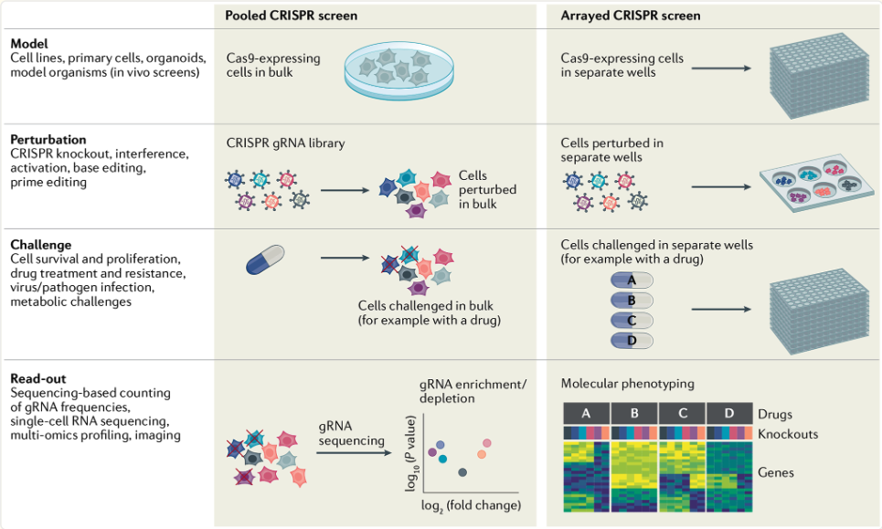
See Figure 8.9 for variations of a CRISPR screen. What we’re discussing more in this chapter is a pooled CRISPR screen.
8.1.1 CRISPR in the wet lab: Design and delivery
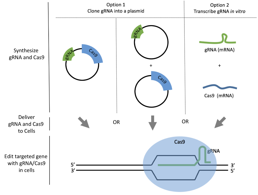
CRISPR experiments begin with the design of a single-guide RNA (sgRNA) that matches the target DNA sequence adjacent to a protospacer-adjacent motif (PAM), which is required for Cas9 recognition and cleavage. The choice of target site is crucial, as off-target effects can lead to unintended mutations. Computational tools such as CRISPOR (Concordet and Haeussler 2018) help predict sgRNA efficiency and minimize off-target binding.
Once the sgRNA is designed, it must be delivered into cells alongside the Cas9 enzyme. This can be achieved, such as using viral vectors such as lentivirus. Viral delivery is particularly useful for stable genome integration in cell populations, while other transient delivery methods allow for temporary gene editing effects. The choice of delivery method depends on the cell type, efficiency, and experimental goals. In single-cell studies, lentiviral vectors are often used to introduce a pooled library of sgRNAs, enabling large-scale CRISPR screens across thousands of individual cells.
8.1.1.1 Commonly used cells.
K562 cells, a human myelogenous leukemia cell line, are widely used in CRISPR screens due to their ease of culture, high transfection efficiency, and well-characterized genome. These cells exhibit an undifferentiated hematopoietic phenotype, making them a valuable model for studying gene regulation, hematopoiesis, and drug resistance. Their high proliferative capacity and ability to grow in suspension allow for efficient perturbation experiments at scale. Additionally, K562 cells have been used extensively in studies involving transcriptional regulation due to their rich chromatin accessibility data from ENCODE, which facilitates the identification of enhancer-gene interactions.
Another one I’ve seen quite often is Jurkat cells. This is a human T-cell leukemia cell line that serves as a model for immunology and T-cell signaling studies, often used in CRISPR screens focused on immune response and checkpoint regulation.
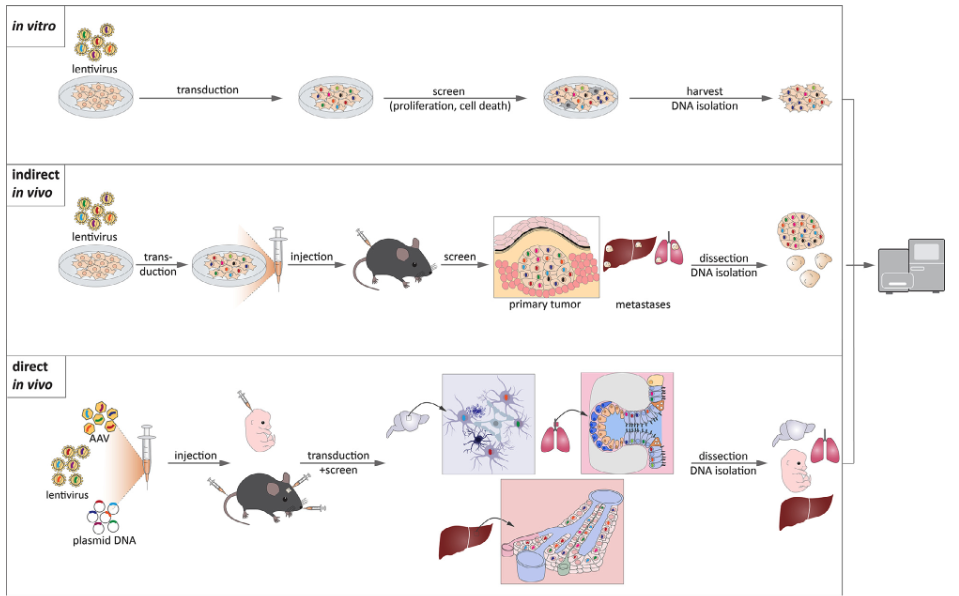
While CRISPR screens are widely applied in established cell lines, extending them to other cell types requires careful experimental planning. Primary cells and non-transformed cell types often have lower transfection or transduction efficiencies, necessitating optimization of delivery methods such as electroporation or viral transduction. Additionally, cell-type-specific chromatin accessibility and DNA repair mechanisms can influence CRISPR efficiency and editing outcomes, requiring tailored guide RNA design and validation. Growth rate and population doubling time must also be considered, as slow-dividing or non-dividing cells may require prolonged selection periods or alternative screening strategies, such as inducible CRISPR systems. Finally, proper negative controls and lineage-specific reference datasets are critical to ensure accurate interpretation of perturbation effects in novel cellular contexts. While most CRISPR screens are done in vitro, there are also technical challenges (which can be controlled for) for in vivo systems, see Figure 8.10.
8.1.2 The jungle of CRISPR: CRISPR-KO, CRISPRi, and CRISPRa
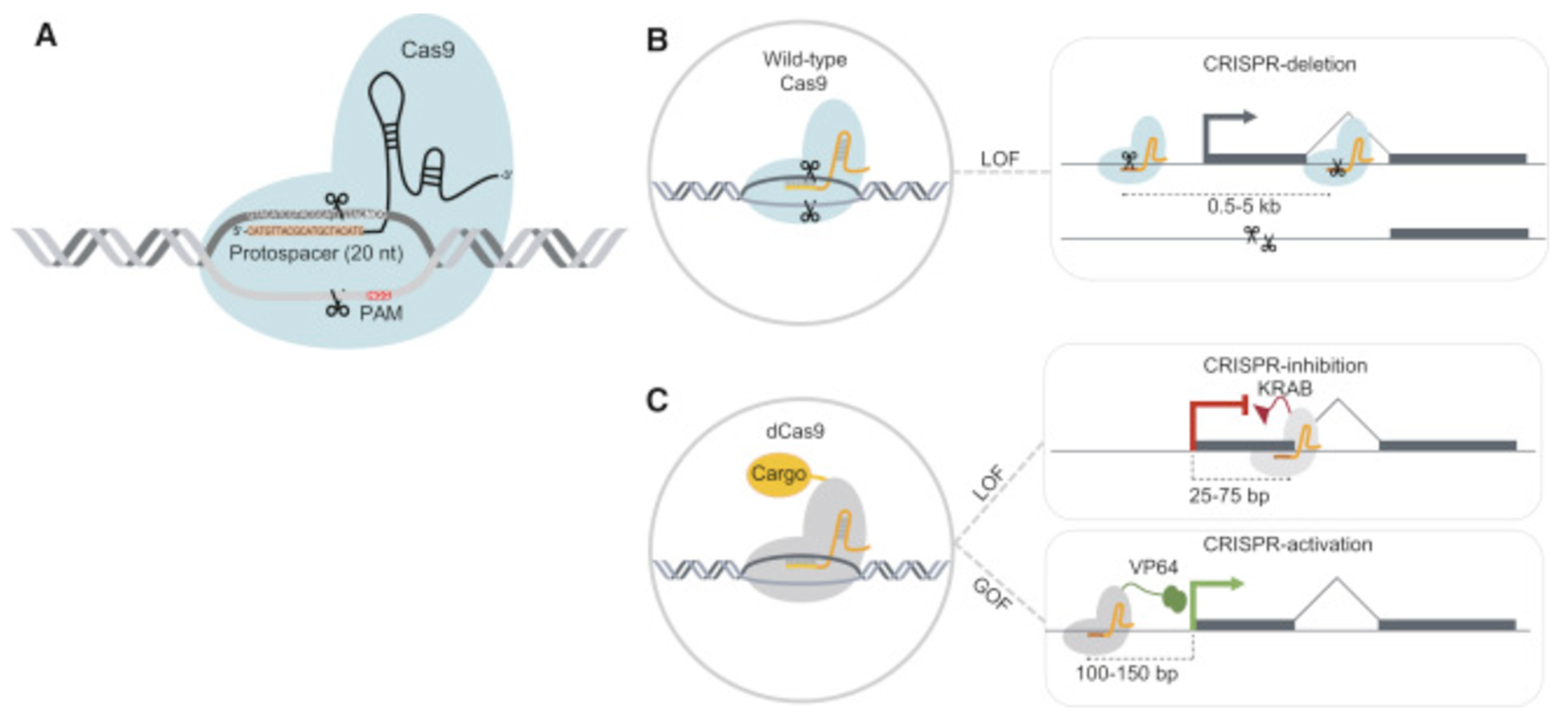
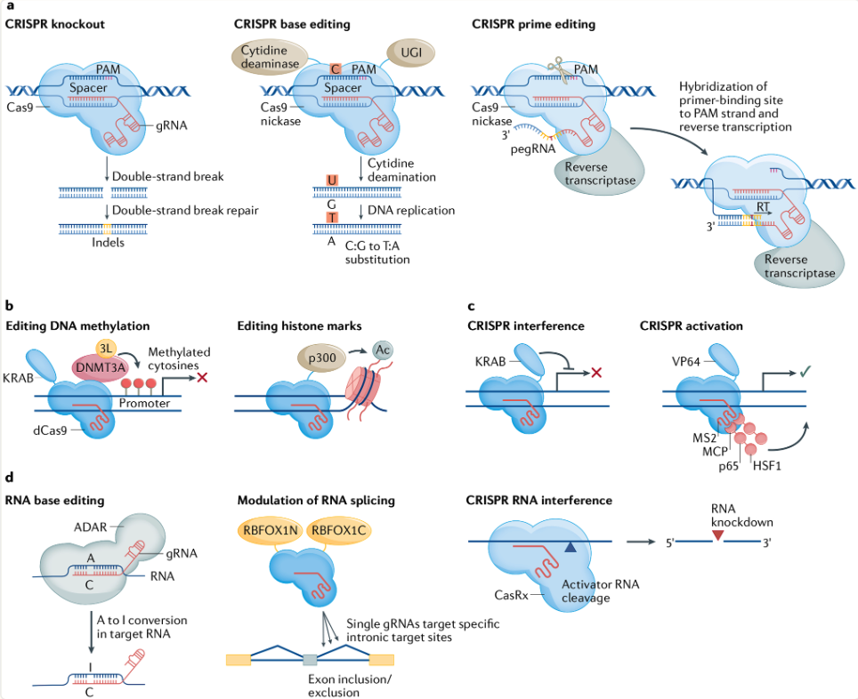
CRISPR can be adapted for different functional purposes beyond simple gene knockout (KO). CRISPR-knockout (CRISPR-KO) involves the use of Cas9 to introduce double-stranded breaks at the target locus, leading to insertions or deletions (indels) that disrupt gene function, which is mainly what we’ve discussed above. This method is widely used for loss-of-function studies to investigate gene essentiality and pathway regulation.
In contrast, CRISPR activation (CRISPRa) and CRISPR interference (CRISPRi) enable gene expression modulation without altering the DNA sequence. CRISPRa employs a catalytically inactive Cas9 (dCas9) fused to transcriptional activators to enhance gene expression. Conversely, CRISPRi uses dCas9 fused to repressive domains such as KRAB to inhibit transcription. These methods allow for fine-tuned control over gene expression levels, making them particularly useful for studying gene regulatory networks at the single-cell level.
See Figure 8.11 and Figure 8.12 for examples of variations of CRISPR screens.
8.1.3 CRISPR screens and single-cell gene expression analysis
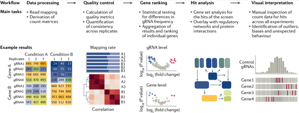
CRISPR screening is a high-throughput approach that uses pooled single-guide RNA (sgRNA) libraries to systematically perturb thousands of genes in a single experiment. There are two main types of CRISPR screens: positive selection screens, which identify sgRNAs that promote cell survival or proliferation, and negative selection screens, which identify essential genes by tracking sgRNAs that are depleted over time. When combined with single-cell RNA sequencing (scRNA-seq), CRISPR screens can reveal gene regulatory interactions at the resolution of individual cells, enabling functional genomics studies at an unprecedented scale. See Figure 8.13 for the bulk-level analysis that does not include RNA-sequencing – this is to give you a sense of the simplistic CRISPR analysis.
To analyze CRISPR perturbations in a single-cell context, cells are first transduced with a pooled sgRNA library, followed by scRNA-seq to capture transcriptomic changes. The identity of the sgRNA in each cell must also be determined in order to link gene perturbations to expression changes. This is typically done through targeted sequencing of the sgRNA cassette embedded in the transcriptome. However, sequencing the guide RNAs presents a challenge because they lack poly-A tails, which are typically required for capture in common scRNA-seq protocols. To overcome this, specialized methods such as Perturb-seq (Dixit et al. 2016) and CROP-seq (Datlinger et al. 2017) incorporate modifications to ensure efficient capture of sgRNA sequences. For example, Perturb-seq integrates the sgRNA into a polyadenylated transcript, allowing it to be captured along with mRNA molecules during reverse transcription.
Computational tools, which we will discuss in Section 8.2, are commonly used to analyze CRISPR screen data by linking sgRNA-induced perturbations to gene expression changes. These tools help identify differentially expressed genes in response to specific genetic perturbations, revealing functional interactions within cellular networks. By combining CRISPR-based gene perturbation with single-cell transcriptomics, researchers can systematically dissect gene function, uncover regulatory networks, and study cellular heterogeneity in response to genetic modifications.
8.1.4 Interpreting CRISPR data and experimental considerations
CRISPR datasets in single-cell studies typically consist of expression matrices where each row corresponds to a gene and each column represents a cell, with additional metadata indicating the sgRNA assigned to each cell. One key challenge in analyzing these datasets is ensuring that each cell receives a single sgRNA, as multiple perturbations can introduce confounding effects. Additionally, technical noise in single-cell RNA sequencing, such as dropout events and variability in sequencing depth, must be accounted for in downstream analyses.
While CRISPR has revolutionized functional genomics, several caveats remain. Off-target effects can complicate result interpretation, requiring careful validation with orthogonal approaches such as RNA interference (RNAi) or small molecule inhibitors. Moreover, certain genes may be difficult to perturb due to low sgRNA efficiency or compensation from redundant pathways.
8.1.4.1 More considerations and readings about CRISPR.
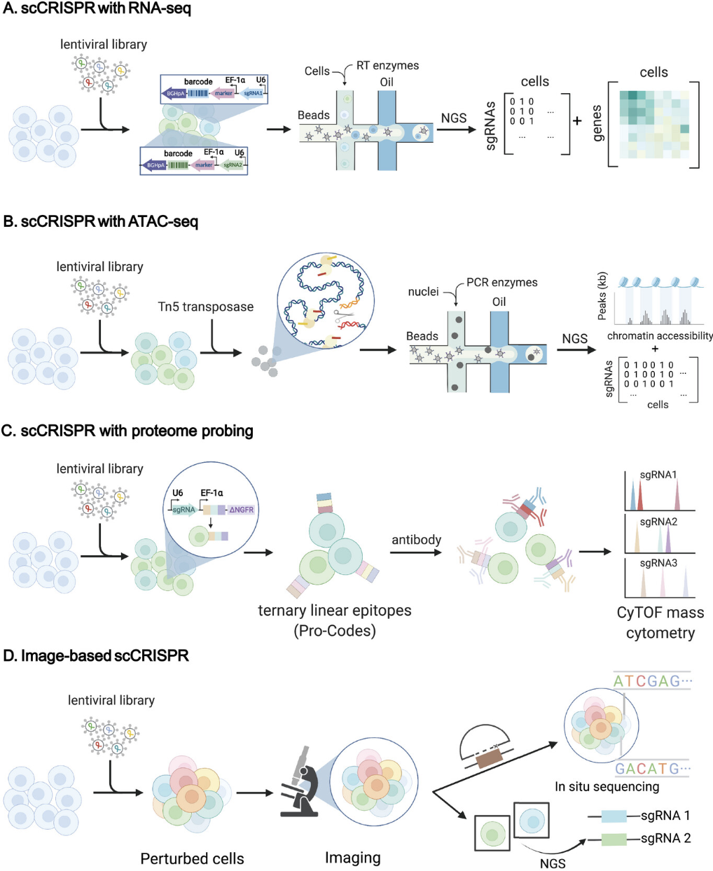
See Bock et al. (2022) for an important checklist (Box 1) to give you a sense the complexities when setting up a CRISPR experiment. Also, keep in mind that many CRISPR experiments are not measuring single-cell gene expressions. However, also (as mentioned above), there are also many CRISPR protocols to measure various omics at single-cell resolution alongside the gRNAs, see Figure 8.14.
For more reading: - https://www.idtdna.com/pages/education/decoded/article/overview-what-is-crispr-screening is probably one of the most helpful webpages I came across.
8.2 Linking gRNA (i.e., perturbations) to its downstream genes
Understanding the causal relationships between genetic perturbations and gene expression changes is a fundamental problem in genomics. Single-cell CRISPR screening technologies enable high-throughput profiling of transcriptomic changes induced by targeted genetic modifications at a single-cell resolution. The goal of the statistical analysis here is to identify genes whose expression levels are significantly altered by specific perturbations, providing insights into gene regulatory networks and functional genomics. However, accurately estimating these effects requires sophisticated statistical methodologies that can properly account for measurement noise, technical confounders, and the stochastic nature of gene expression.
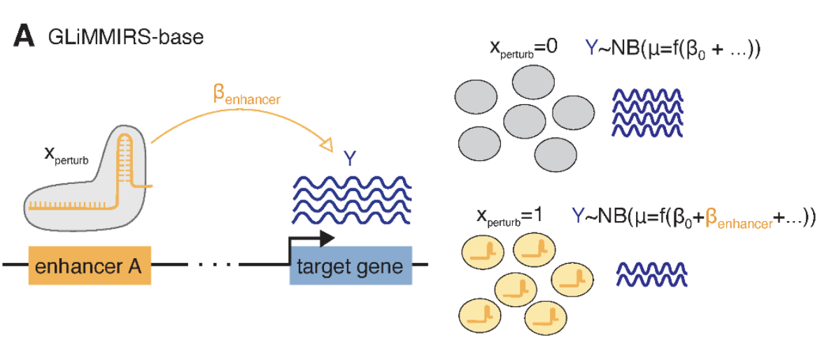
A prototypical statistical model for this analysis is based on a generalized linear model (GLM) or a negative binomial regression framework, where gene expression levels are modeled as a function of perturbation status, along with potential confounders such as sequencing depth, batch effects, and cellular state, see Figure 8.15. Here are some statistical challenges a typical statistical method might account for:
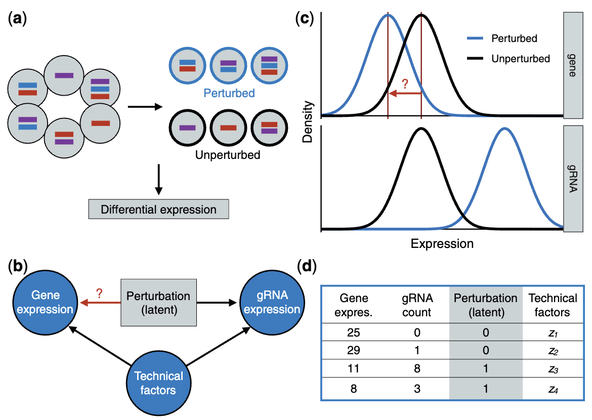
- Inferring which cells got which perturbation: Given that perturbations are not directly observed but inferred through guide RNA (gRNA) expression, a crucial modeling step involves using a measurement error framework or latent variable model to impute perturbation identities. The presence of background noise in gRNA detection complicates direct classification of perturbed versus unperturbed cells. See Figure 8.16.
- Account for unmeasured confounders: Variations in sequencing efficiency or cell cycle effects (i.e., unmeasured biological processes that affect both the guide RNA and gene expression) can introduce spurious associations between perturbations and gene expression if not properly adjusted
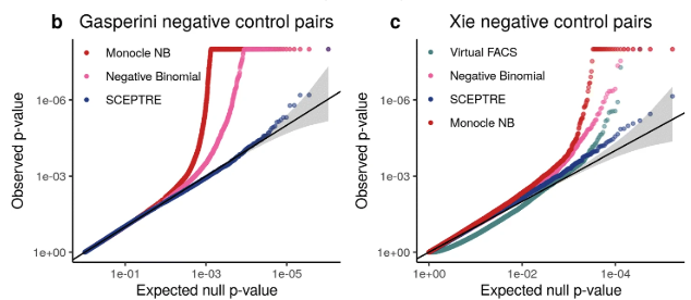
Fortunately, one experimental consideration we can use to advantage are negative control perturbations – perturbations that target non-functional genomic regions. These provide a null distribution against which true perturbation effects can be compared. Certain methods can use the negative controls to calibrate the p-values, while others use the negative controls to validate their control of false discovery rates.
The goal of this analysis is produce a p-value for every sgRNA (targeting an enhancer) and gene pair. This is often visualized a QQ-plot, shown in Figure 8.17.
8.2.0.1 A typical choice: SCEPTRE.
SCEPTRE (Barry et al. 2021) (Analysis of single-cell perturbation screens via conditional resampling) is a statistical method designed to analyze gene-gRNA associations in single-cell CRISPR screens. It distinguishes true regulatory relationships from spurious ones by properly accounting for confounding technical factors and by circumventing strict parametric assumptions.
Input/Output. The input to SCEPTRE is a 1) single-cell gene expression count matrix \(Y\in \mathbb{Z}_+^{n\times p}\) for \(n\) cells and \(p\) genes, and 2) a single-cell guide RNA count matrix of the same \(n\) cells, \(X \in \{0,1\}^{n\times d}\) for \(d\) perturbations. The output is a pairing between certain \(k\) perturbations and \(p\) genes (not necessarily one-to-one) with associated p-values. We can screen these p-values for significant ones after multiple-testing correction to determine which perturbations are associated (but not necessarily statistically causal in this method) with which genes.
Are the guide RNAs measured as binary or counts?
SCEPTRE “thresholds” the gRNA count matrix to be a binary matrix (i.e., which cells received which perturbation). However, in reality, this information is itself sequenced and can be noisy. The authors then wrote a follow-up paper called GLM-EIV (Barry, Roeder, and Katsevich 2024) to further account for this.
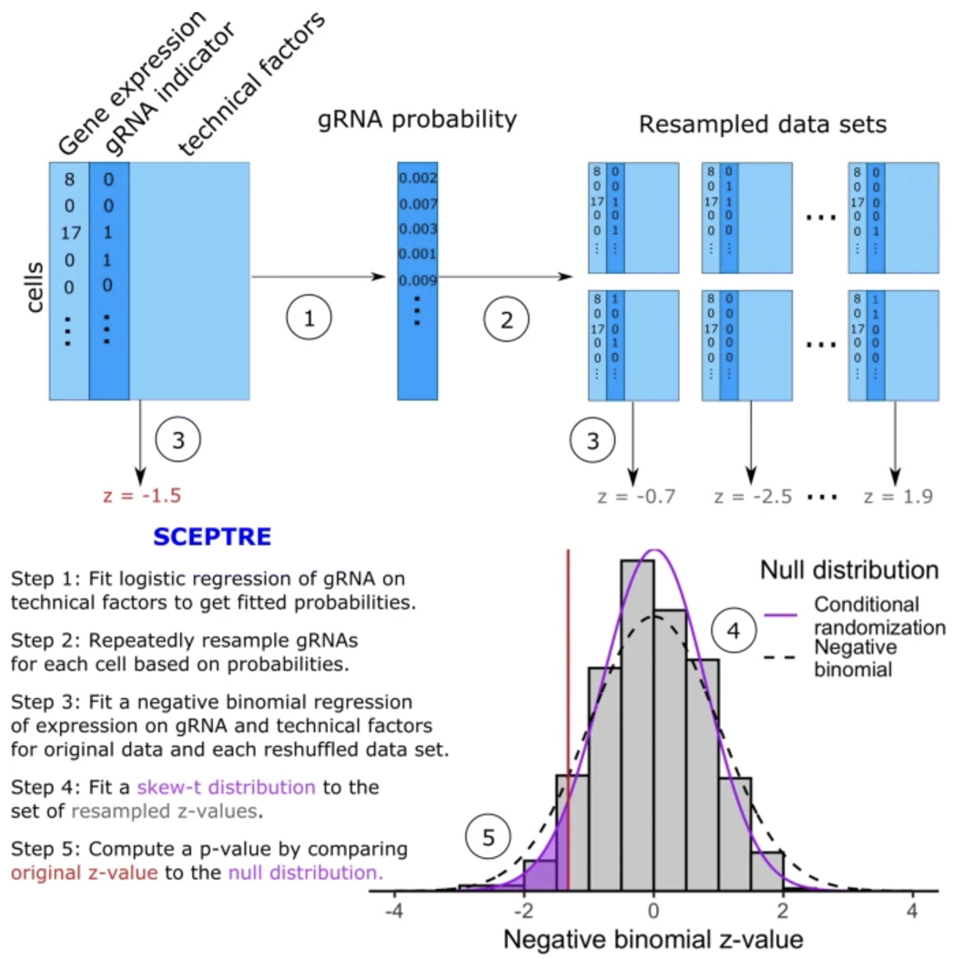
We describe the main components of SCEPTRE below. See Figure 8.18 for an illustration of this method.
Input Data. Let \(n\) be the number of cells, \(p\) the number of genes, and \(k\) the number of gRNAs. The gene expression data can be represented by an \(n \times p\) matrix, where each entry \(Y_{ij}\) is the observed count (for instance, UMI count) of gene \(j\) in cell \(i\). The gRNA detection data can be represented by an \(n \times d\) binary matrix, where each entry \(X_{ik}\) indicates whether gRNA \(k\) was observed in cell \(i\) (commonly treated as a binary indicator). In addition, each cell \(i\) has a vector of technical covariates \(Z_i \in \mathbb{R}^r\) (for instance, capturing batch, sequencing depth, or other factors). These covariates are crucial, as they can affect both the probability of detecting a given gRNA and the observed gene expression counts.
Negative Binomial Expression Model. To test the association between a particular gene \(j\) and gRNA \(k\) (typically within 1 Mb apart), consider one-dimensional slices \(Y_i\) and \(X_i\), denoting that cell \(i\) has count \(Y_i\) for gene \(j\) and \(X_i \in \{0,1\}\) for gRNA \(k\). A typical regression model is
\[ Y_i \sim \mathrm{NegBin}(\mu_i, \alpha), \quad \log(\mu_i) = \beta_0 + \beta \, X_i + \gamma^\top Z_i, \]
where \(\alpha\) is a dispersion parameter, \(\beta\) measures how the presence of the gRNA (\(X_i\)) shifts the mean expression \(\mu_i\), and \(\gamma\) captures the effect of the technical covariates. Fitting this negative binomial regression provides a test statistic, for example a \(z\)-score \(T = \beta / \text{SE}(\beta)\), that quantifies the strength of the association between \(X_i\) and \(Y_i\).
- Logistic Model for gRNA Detection. A key insight in SCEPTRE is that \(X_i\) itself is subject to measurement variability and is influenced by the same covariates \(Z_i\). This can be modeled via
\[ \pi_i = P(X_i = 1 \mid Z_i), \quad \log\!\Bigl(\frac{\pi_i}{1 - \pi_i}\Bigr) = \tau_0 + \tau^\top Z_i. \]
Fitting this logistic model to the observed gRNA indicators provides estimated probabilities \(\hat{\pi}_i\) for each cell.
- Conditional Resampling. SCEPTRE constructs an empirical null distribution by repeatedly resampling “fake” gRNA indicators \(\tilde{X}_i\) in each cell, drawn independently from \(\mathrm{Bernoulli}(\hat{\pi}_i)\). In each resampled dataset, one holds \(Y_i\) and \(Z_i\) fixed but replaces the original \(X_i\) with \(\tilde{X}_i\). For each resample, one refits the negative binomial regression (using an efficient shortcut) to compute a new test statistic \(\tilde{T}\). The empirical distribution of these \(\tilde{T}\) values represents how the test statistic would behave under the null hypothesis (no real regulatory effect) but with confounders preserved. The SCEPTRE \(p\)-value compares the actual test statistic \(T\) against this resampling-based distribution, thus ensuring valid inference even if the negative binomial model for \(Y_i\) is not perfectly specified.
This is a common statistical trick. Essentially, the idea is: we constructing “fake” gRNA data that accounts for the technical factors but we are guaranteed to not relate to gene expression (thanks to how we sampled this fake data). Then, we can use this “fake” data to see what the typical estimated relation between the gRNA and gene is. We deem a gRNA and gene as a significant pair if the estimated relation is stronger than this “fake” distribution.
8.3 Estimating gene pathways impacted by a group of perturbations
Understanding the impact of CRISPR-based genetic perturbations on gene expression requires methods that can accurately capture coordinated transcriptional responses. Rather than affecting single genes in isolation, many perturbations influence entire regulatory networks or gene modules. Grouping genes and guide RNAs (gRNAs) into functional modules provides a structured framework to infer how perturbations propagate through cellular pathways, enhancing the ability to detect meaningful biological signals. See Dixit et al. (2016) and Schnitzler et al. (2024) for analyses that performed this type of analysis.
Biologically, grouping genes into modules is motivated by the observation that genetic perturbations often target key regulatory elements such as transcription factors, chromatin remodelers, or signaling pathway components. These elements control multiple downstream genes, making it crucial to infer their collective effects rather than analyzing genes independently. Single-cell CRISPR screens allow for the systematic interrogation of gene regulatory networks, but sparsity in the data and limited per-perturbation cell numbers necessitate statistical techniques that integrate information across functionally related genes. Here are some statistical challenges (very similar to the ones introduced in Section 8.2).
Sparse and noisy guides: Perturbation effects are often sparse, meaning that each perturbation affects only a subset of genes, necessitating regularized models that can extract meaningful structure from noisy data. Also, single-cell CRISPR screens require inference of perturbation identities, as not all cells successfully receive a gRNA, and sequencing-based methods introduce detection noise.
Unmeasured confounders: Batch effects, cell cycle states, and sequencing depth variations, can obscure true biological signals, making it essential to employ factor models that account for these sources of variability.
Higher MOI for cheaper sequencing costs: A complexity arises when analyzing interactions between perturbations. Many CRISPR screens employ pooled designs where multiple perturbations may be present within the same cell. This can introduce nonlinear effects or epistatic interactions, where the combined influence of two perturbations deviates from the sum of their individual effects. See Yao et al. (2024) and Lin et al. (2022) for some examples of this.
8.3.0.1 A current choice: GSFA.
Guided Sparse Factor Analysis (GSFA) (Y. Zhou et al. 2023) is a Bayesian approach to analyze single-cell CRISPR screens, where multiple genetic perturbations (gRNAs) and whole-transcriptome gene expression are measured across individual cells. Below is a concise description of its components, using more detailed notation. (There is no commonly agreed upon method for this analysis at this time. You should think of GSFA as a promising start of a sequence of research. Future methods might account for guide RNA efficiency, non-additive effects, bioinformatics between guide RNA and target genes, etc.)
Input/Output. The input to GSFA is a 1) single-cell gene expression count matrix \(Y\in \mathbb{R}^{n\times p}\) for \(n\) cells and \(p\) genes, and 2) a single-cell guide RNA count matrix of the same \(n\) cells, \(G \in \{0,1\}^{n\times d}\) for \(d\) perturbations. Here, \(Y_{ij}\) is the normalized expression of gene \(j\) in cell \(i\). The output of GSFA are: 1) a matrix \(W \in \mathbb{R}^{p \times k}\) that denotes which genes is in which module (i.e., latent factor), and 2) a matrix \(\beta \in \mathbb{R}^{d \times k}\) that denotes which perturbation is in which module.
We describe the main components of GSFA below. See Figure 8.19 for an illustration of this method.
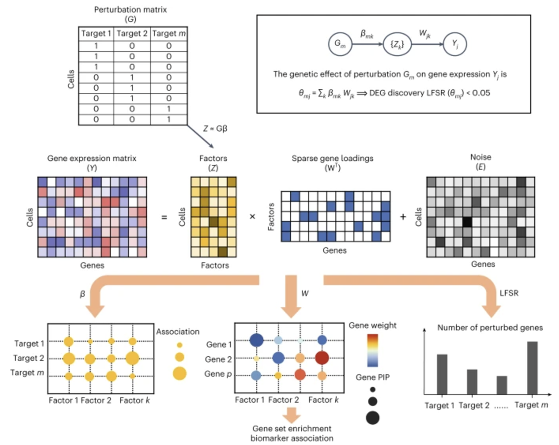
- Nested matrix factorization model: GSFA decomposes the expression matrix into latent factors \(Z\) and gene loadings \(W\), while modeling how these factors depend on \(G\):
\[ \underbrace{Y_{ij}}_{\text{Expression}} = \sum_{\ell=1}^k Z_{i\ell}\,W_{j\ell} + E_{ij}, \qquad \underbrace{Z_{i\ell}}_{\text{Factors}} = \sum_{m=1}^d G_{im}\,\beta_{m\ell} + \phi_{i,k}. \]
Here, \(k\) is the number of latent factors, \(E_{ij}\) is residual noise (often assumed Gaussian), and \(\phi_{i\ell}\) is a Gaussian random term that captures variation in factor \(\ell\) not explained by perturbations. The factors \(Z_{i\ell}\) can be interpreted as “gene modules” or “principal axes” of variation in the single-cell data.
Sparse priors and Bayesian inference: Each perturbation \(m\) is assumed to affect only a few latent factors, reflected in a sparse prior on the effect sizes \(\beta_{m\ell}\). Similarly, each factor \(\ell\) is assumed to influence only a small subset of genes, reflected in a sparse prior on \(W_{j\ell}\). These priors impose the idea that genetic perturbations typically alter only a limited set of biological pathways. GSFA uses Gibbs sampling to draw from the posterior distributions of \(\beta_{m\ell}\), \(W_{j\ell}\), and \(Z_{i\ell}\) given the observed data \((Y, G)\).
Factor association: Once \(Z\) and \(\beta\) are estimated, GSFA identifies which gRNAs significantly shift which factors. The parameter \(\beta_{m\ell}\) measures how strongly perturbation \(m\) activates or represses factor \(\ell\). Posterior inclusion probabilities (PIPs) are computed to assess confidence in each \(\beta_{m\ell}\) being nonzero.
Gene-level effects: GSFA also summarizes the overall impact of perturbation \(m\) on gene \(j\). Since perturbation \(m\) can affect multiple factors, and each factor influences the expression of gene \(j\), the total effect is
\[ \theta_{mj} = \sum_{\ell=1}^k \beta_{m\ell}\,W_{j\ell}. \]
The distribution of \(\theta_{m,j}\) is sampled under the model’s posterior, yielding an LFSR (local false sign rate) that quantifies significance and sign confidence of the perturbation’s effect on that gene.
In practice, GSFA is applied to single-cell CRISPR screen data as follows. First, one often transforms count data (for example, via deviance residuals) and centers/scales covariates. Next, one fits GSFA via Gibbs sampling, obtaining posterior samples of the factors, gene loadings, and perturbation-factor effects. The factor discovery step can reveal broad biological modules (cell-cycle, immune response, neuronal development, etc.), while the gene-level effect summaries \(\theta_{mj}\) yield a differential expression–style list of significantly perturbed genes for each gRNA. By borrowing information across genes that move together, GSFA can be more sensitive than a naive single-gene test, and can better separate real signals from confounding or measurement noise.
8.3.0.2 A brief note about other work.
Schnitzler et al. (2024) demonstrates using CRISPR to link SNPs in a GWAS to the regulated genes. (This paper also mentions a consensus NMF, which illustrates a different variation of clustering genes by regulatory pathways.) Yao et al. (2024) demonstrates a method to “unravel” the effect of each perturbation on genes in high MOI experiments, where there are multiple perturbations purposely placed in cell, or multiple cells purposely placed in each droplet.
8.4 Prediction perturbation effects (for CRISPR screens, but other types of perturbations as well)
A fundamental computational challenge in single-cell perturbation studies is predicting how a perturbation, such as a drug treatment or CRISPR-based genetic modification, affects cellular behavior. This challenge arises in two primary contexts: (1) given a perturbation applied to one cell type, where both control and perturbed states are observed, inferring how another cell type would respond to the same perturbation based on its unperturbed expression; or (2) disentangling the latent space of perturbations from the latent space of cell embeddings, allowing for generalizable predictions of perturbation effects even in the absence of direct observations. The latter approach leverages biological priors on perturbation relationships, enabling the extrapolation of perturbation effects across unseen conditions. Accurate prediction methods are crucial for understanding drug responses, genetic knockouts, and CRISPR-based enhancer perturbations, ultimately providing insights into gene regulatory networks and therapeutic interventions.
8.4.0.1 Hold on… Why do we need this again?
Remember: If we use a low MOI (ex: MOI of 0.3) experiment, we need many cells to receive each guide, and we even more cells because most cells won’t receive a guide. To quote Bock et al. (2022),
“For both genome-scale and focused CRISPR knockout (CRISPRko) screens, it is advisable to include at least four different gRNAs for each target gene, although carefully designed and validated gRNA libraries with fewer gRNAs per gene can provide reliable results. All gRNA libraries should include gRNAs for application-specific positive and negative control genes, which are important to validate the screen. In addition, they should include control gRNAs that target known safe harbour loci or other genomic regions where no specific effects of gene editing are expected, in order to account for the DNA damage response and for non-specific reduction in cell proliferation caused by CRISPRko. …
As a guideline, we recommend a coverage of 100-200 cells per target gene for positive selection screens and 500-1,000 cells per target gene for negative selection screens.”
(The reason negative selection screens need more cells is because these cells will die from the stressor after the CRISPRko integration. So you need to be confident these cells really “died” (instead of you happening by bad luck to miss these cells during sequencing).)
For this reasons, some CRISPR experiments purposely use a high MOI (think of 10 to 50). This reduces the number of cells they need, since most cells will receive multiple guides. As one concrete example, see Gasperini et al. (2019), which performed a CRISPRi screen. They targeted 1,119 candidate enhancer elements (which was near 5,611 genes) in K562 cells, and used a high MOI (roughly 15) across 47,650 cells. This means, if they used a conservative MOI=1 (i.e., each cell receives only one guide), they would needed about \(47,650 \times 15 \approx 715,000\) cells. (That would make that experiment a massive (and extremely expensive) single-cell experiments.)
However, the drawback of high MOI is that sometimes you cannot reasonably rule that different sgRNA doesn’t interact with one another. For this reason, we might wonder: Can we: 1) use a low MOI experiment, 2) leverage some biological insights about these sgRNA, and 3) develop a fancy computational tool to synthetically predict what the effects of the sgRNA we didn’t actually use are?
8.4.0.2 Brief aside: What on earth is a “normalizing flow neural networks”?
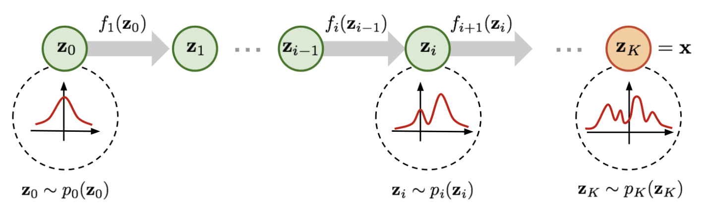
Normalizing flow neural networks provide a framework to construct a rich, complex probability distribution by applying a series of invertible transformations to a simple base distribution (often a Gaussian), see Figure 8.20 and Figure 8.21. Each transformation is designed to be bijective and differentiable, which ensures that the overall mapping from the latent space to the data space remains invertible. This property allows for exact likelihood evaluation, because the change of variables formula can be applied directly to the transformed distribution. In practice, one computes the log-likelihood of an observed sample by summing the log of the Jacobian determinant of each invertible mapping and the log-likelihood of the base distribution.
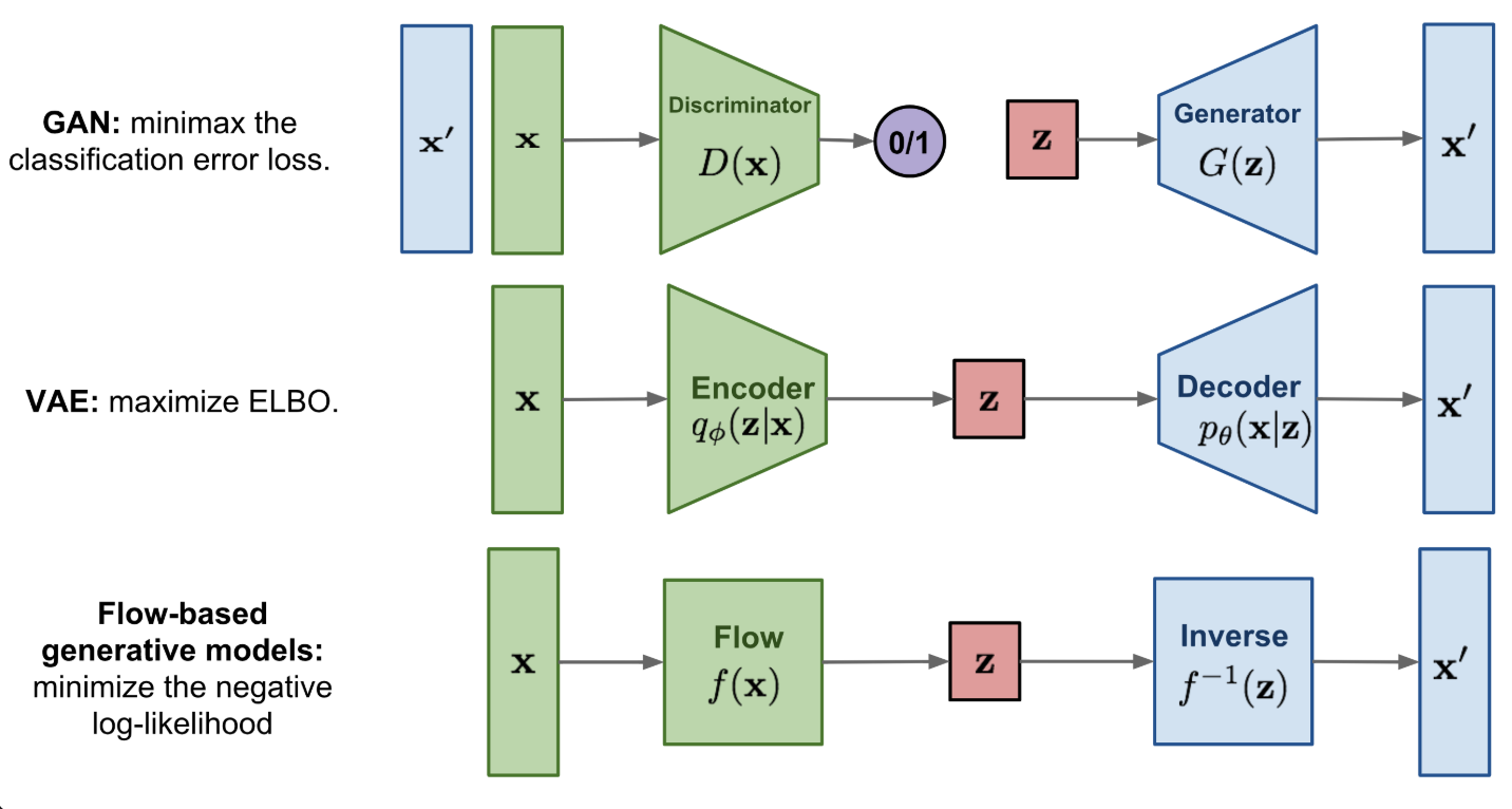
Invertibility is a key difference between normalizing flows and Variational Autoencoders (VAEs). In a VAE, an encoder approximates a posterior distribution over the latent variables, but it is generally not invertible. Consequently, VAEs compute a lower bound of the log-likelihood rather than the exact likelihood. In contrast, the invertible nature of normalizing flows enables direct calculation of the log-likelihood, thereby avoiding the need for variational approximations. This leads to more precise density estimation and can offer a clearer interpretation of how each layer transforms data.
Here is one concrete example of what a normalizing flow network is, which is called RealNVP (where NVP stands for “non-volume preserving”). RealNVP (Dinh, Sohl-Dickstein, and Bengio 2016) is a type of invertible (or “normalizing flow”) model where each transformation can be inverted cheaply by design. The primary idea is to split the input vector \(\mathbf{x}\) into two parts, keep one part unchanged (\(\mathbf{x}_1\)), and transform the other part (\(\mathbf{x}_2\)) in a way that is guaranteed to be invertible.
- Coupling Layer: Partition \(\mathbf{x}\) into \(\mathbf{x}_1\) and \(\mathbf{x}_2\). Then, define the output \(\mathbf{y} = (\mathbf{y}_1, \mathbf{y}_2)\) where \(\mathbf{y}_1 = \mathbf{x}_1\) and
\[ \mathbf{y}_2 = \mathbf{x}_2 \,\odot\, \exp\bigl(\mathbf{s}(\mathbf{x}_1)\bigr) + \mathbf{t}(\mathbf{x}_1). \]
The functions \(\mathbf{s}(\cdot)\) and \(\mathbf{t}(\cdot)\) can be any neural networks that output real-valued vectors. The exponential ensures a nonzero scale factor, while addition by \(\mathbf{t}\) is trivially invertible. See Figure 8.22.
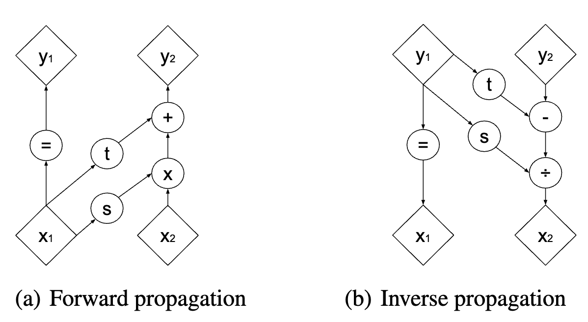
- Ensuring this transformation is invertible: The inverse of the above transformation is
\[ \mathbf{x}_1 = \mathbf{y}_1, \quad \mathbf{x}_2 = \bigl(\mathbf{y}_2 - \mathbf{t}(\mathbf{y}_1)\bigr) \,\odot\, \exp\bigl(-\mathbf{s}(\mathbf{y}_1)\bigr). \]
Because \(\mathbf{x}_1\) remains the same, it is straightforward to reconstruct \(\mathbf{x}_2\). No matter how \(\mathbf{s}\) and \(\mathbf{t}\) are learned, the coupling layer is invertible by construction.
Splitting the input and only transforming part of it guarantees efficient forward and inverse computations. By composing multiple coupling layers, we can create flexible density estimators while preserving tractable log-likelihood calculation.
See https://lilianweng.github.io/posts/2018-10-13-flow-models/, https://paperswithcode.com/method/affine-coupling, https://bjlkeng.io/posts/normalizing-flows-with-real-nvp/, and Kobyzev, Prince, and Brubaker (2020) for useful overviews about normalizing flows, with some details about the way to construct normalizing flows using affine transformations.
(Sidenote: This context is mainly only needed to understand PerturbNet (Yu and Welch 2022). There are plenty of methods to predict perturbation effects not build using normalizing flow networks. See scGen (Lotfollahi, Wolf, and Theis 2019) for example, which is built on your more typical VAE architecture.)
8.4.0.3 State-of-the-art research: PerturbNet.
PerturbNet (Yu and Welch 2022) is a deep generative framework that predicts single-cell gene expression responses under both observed and unseen chemical or genetic perturbations. That is, we want to predict the effect of perturbation even if none of cells ever received this perturbation.
Input/Output. The input to PerturbNet (when trying to perturb the impact of CRISPRi perturbations) is a 1) single-cell gene expression count matrix \(\mathbb{Z}_+^{n\times p}\) for \(n\) cells and \(p\) genes, 2) a single-cell guide RNA count matrix of the same \(n\) cells, \(\{0,1\}^{n\times d}\) for \(d\) perturbations, and 3) a database that groups the perturbations (many of which might not the \(d\) perturbations you actually measured) into pathways. The output is three things: 1) a VAE to embed each of the \(n\) cells into low-dimensional space, 2) a VAE to embed each of the perturbations (including the \(d\) in your dataset) into a low-dimensional space, and 3) a learned function that takes in a cell’s latent representation and perturbation’s latent representation and outputs the (predicted) cell’s latent representation after receiving that perturbation.
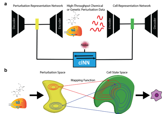
It is designed around three principal building blocks: (i) perturbation representation networks, (ii) cell-state representation networks, and (iii) a conditional invertible neural network (cINN) that translates perturbation embeddings into full distributions of cellular states.
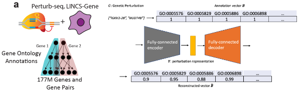
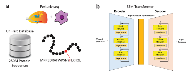
- Perturbation Representation Networks (GenotypeVAE or ESM): To capture key features of chemical or genetic perturbations in a low-dimensional, learnable space, PerturbNet uses different encoder architectures. We’ll just focus on the CRISPR-related perturbations in our discussion here. For CRISPR knockdown or CRISPRi/a perturbations, a GenotypeVAE is used, which starts from a high-dimensional GO-term annotation vector for each target gene (or union of genes), then encodes this vector into a condensed gene-function latent space via fully-connected layers. In the case of coding-sequence edits (such as CRISPR knockouts which introduce changes to the genetics), perturbations are encoded by a pretrained transformer (e.g. ESM, which stands for “evolutionary scale modeling”3), which outputs a deterministic embedding of amino-acid sequences.
The point is: we use biological insights about these perturbations (which use established databases) to learn the “space of perturbations.” See Figure 8.23 and Figure 8.24.
Cell-state representation network: Separately, PerturbNet learns a latent space for the single-cell gene expression profiles. This is similar to your typical VAE for scRNA-seq using a negative binomial-likelihood. Each cell is thus mapped into a latent space \(Z\) capturing core variation in gene expression. The VAE decoder reconstructs the input (e.g. counts) from the sampled \(Z\) latent, enabling distributional modeling of single-cell data.
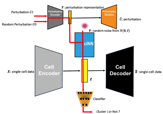
Conditional invertible neural network (cINN): [[This is where the magic happens!]] The crux of PerturbNet is a conditional invertible neural network, denoted \(Z=f(V \mid Y)\). (This is where the normalizing flow comes into play.) Here, \(Y\) is the perturbation’s latent embedding (from GenotypeVAE or ESM), and \(Z\) is the cell-state latent (from the cell VAE). The cINN incorporates a “residual” variable \(V \sim N(0,I)\), capturing per-cell variability unexplained by the perturbation. In plain English, you want learn the function \(f\) that takes in as input \(V\) (the “baseline” representation of the cell), and then condition to a perturbation (represented by \(Y\)) to give you the observed gene expression (which here, is a low-dimensional embedding represented by \(Z\)).
Concretely, \(f\) is built from affine coupling blocks (see Figure 8.22):
\[ (W_1, W_2) = \mathrm{Block}((U_1,U_2) \mid Y), \]
where \(U_1,U_2\) split the input, and each block’s parameters are learned via fully-connected sub-networks that shift and scale one part of the data conditioned on the other part and on \(Y\). Because each block is invertible (with a tractable Jacobian determinant), one can train \(f\) from the objective4
\[ \mathcal{L} = \mathbb{E} \bigl[-\log p\{f^{-1}(Z \mid Y)\}\bigr] + \text{(constant terms)}, \]
driving \(f^{-1}\) to map \((Z,Y)\) back to a Gaussian \(V\). (I’m aware this probably doesn’t make a lot of sense since I’m not providing enough context about how a cINN works. See the references above about normalizing flows.)
This cINN architecture thus learns to sample realistic cell embeddings for each perturbation. In practice, a stack of multiple affine coupling blocks plus normalization layers is used, ensuring expressivity and stable training.
- Training procedure and use: After the perturbation and cell VAEs are pre-trained (often on large unpaired datasets), one collects paired perturbation–cell data (e.g. a high-throughput Perturb-seq or chemical screen). By feeding the latent \(Y\) from the perturbation network and the latent \(Z\) from the cell-state VAE into the cINN, PerturbNet learns the probabilistic mapping between \(Y\) and \(Z\). Once trained, it can (1) sample predicted single-cell states for a new perturbation \(Y_{\mathrm{new}}\), and (2) be inverted to find which perturbation embeddings shift cells toward a desired \(Z_{\mathrm{target}}\) distribution.
Putting this all together, see Figure 8.25 and Figure 8.26.
CRISPR stands for “clustered regularly interspaced short palindromic repeats,” but it’s not too important to know why exactly it’s called this for the purposes of this chapter.↩︎
Transfection is the process of introducing foreign nucleic acids (such as DNA or RNA) into eukaryotic cells to manipulate gene expression or enable genetic modifications. It is commonly used in plasmid-based CRISPR applications. In opposition, transduction refers to the introduction of genetic material using viral vectors..↩︎
This itself is fascinating. See https://github.com/facebookresearch/esm.↩︎
Here, the probability \(p\) is determining the likelihood \(f^{-1}(Z \mid Y)\) originated from \(V \sim N(0,I)\). We’re going to approximate the expectation by taking an average of all the cells we’ve sequenced based on their latent embedding \(Z\) and the latent embedding of the treatment \(Y\) that was applied to that cell.↩︎